Original Article
, Volume: 13( 2)Novel Way of Medical Datasets Classification Using Evolutionary Functional Link Neural Network
1Computer Science Engineering Department, SOA University, Bhubaneswar, Odisha, India
2Information and Communication Technology Department, Fakir Mohan University, Balasore, Odisha, India
- *Correspondence:
- Sahu A, Computer Science Engineering Department, SOA University, Bhubaneswar, Odisha 751030, India, Tel: 06742350635; E-mail: amaresh_sahu@yahoo.com
Received: January 01, 2017; Accepted: March 09, 2017;; Published: March 13,2017
Citation: Sahu A, Pattnaik S. Novel Way of Medical Datasets Classification Using Evolutionary Functional Link Neural Network.Biotechnol Ind J. 2017;13(2):131.
Abstract
Computational time is high for Multilayer perceptron (MLP) trained with backpropagation learning algorithm (BP) also the complexity of the network increases with the number of layers and number of nodes in layers. In contrast to MLP, functional link artificial neural network (FLANN) has less architectural complexity, easier to train, and gives better result in the classification problems. The paper proposed an evolutionary functional link artificial neural network (EFLANN) using genetic algorithm (GA) by eliminating features having little or no predictive information. Particle swarm optimization (PSO) is used as learning tool for solving the problem of classification in data mining. EFLANN overcomes the non-linearity nature of problems by using the functionally expanded selected features, which is commonly encountered in single layer neural networks. The model is empirically compared to FLANN gradient descent learning algorithm, MLP and radial basis function (RBF). The results proved that the proposed model outperforms the other models on medical datasets classification.
Keywords
Functional link artificial neural network; Feature selection; Particle swarm optimization and genetic algorithm
Introduction
Classification task is one of the most important research areas of data mining. A lot of research has focused on the field over the last several years [1-3]. The Data mining is a process of discovering knowledge from large gamut of data. Various classification models in this regard. James has used a linear or quadratic discriminates techniques for solving problems in classification [4]. Another procedure has been employed by using decision trees [5,6]. In the same perspective Duda et al. has proposed discriminant analysis based on the Bayesian decision theory, however he has mentioned traditional statistical models are built mainly on various linear assumptions [7]. To overcome the disadvantage, artificial intelligent tools have been emerged to solve classification problems in data mining. That is why genetic algorithm models were used [8].
Related work
In a recent study, Zhang has introduced the neural networks technique as a powerful classification tool [9,10]. Artificial neural networks (ANNs) have gained extensive popularity in research activities and are generally implemented as a data-based technique in performing nonlinear system identification of complex process. ANNs have been used increasingly as a promising modeling tool in almost all human related activities where quantitative approaches can be used to help in decision making. e.g. functional approximation, rule extraction, pattern reorganization and classification, forecasting and prediction, business, electrical engineering, medical and civil engineering. Multilayer perceptrons (MLPs) are the most common type of neural networks applied successfully for identification and control of a variety of nonlinear processes. Various research activities have been done from Mcculloch-Pitts model of neuron to higher order neuron are considerable with many research papers [11,12]. Feed forward neural networks which based on single layer of linear threshold logic units exhibit fast learning. e.g. the simple perceptron can solve a linearly separable problem in a finite number of learning steps, however, it does not converge or approximate nonlinear decision making problems [13]. By using gradient descent learning algorithm to adjust the weights, adline tries to find a solution which minimize a mean square error criterion [14,15], But its discrimination capability is also limited to linearly separable problems. Many real problems involve approximating nonlinear functions or forming multiple nonlinear decision regions limits the applicability of simple single layered networks of linear threshold unit. By adding of a layer of hidden units dramatically increase the power of layered feed forward networks. In MLP using the back propagation (BP) learning algorithm has been successfully applied to many application problems. However, the training speed of MLPs are typically slower than those for feed forward networks consist of a single layer of linear threshold units due to back propagation of error introduced by multi layering. However, problems occur in MLP training are local minima trapping, saturation, weight interference, initial weight dependence and over fitting. Also, it is very difficult to fix the parameters like number of neurons in a layer and number of hidden layers in a network. So, to decide a proper architecture is difficult. An easy way to avoid the problems is of removing the hidden layers. The removing process should be carried out without giving up non-linearity. Provided that the input layer is en-downed with additional higher order units [16-18]. In other words, higher order correlations among input components can be used to construct a higher order networks to perform nonlinear mapping using only a single layer of units [12,16]. All these indicate the field of HONs like functional link neural networks, pi-sigma neural networks, radial basis functions and polynomial neural networks(RPNNs) [19-30]. A direction is given by Pao et al, that functional links neurons may be conveniently used for function approximation with faster convergence rate and lesser computational load than MLP [31]. FLANN with gradient descent method has achieved good results in classification task of data mining. Also, different set of orthogonal basis functions have been suggested for feature expansion [32]. FLANN is basically a flat network without requiring hidden layers and has simple learning rule. For enhancing the classification accuracy two FLANN based classifiers with genetic algorithms have been developed [33,34]. In FLANN, the dimensionality of input vector is also effectively increased by using functional expansion of the input vector and hence the hyper planes generated by the FLANN providing greater discriminating capability of input patterns. Although FLANN using the gradient descent gives promising results, sometimes it may be trapped in local optimal solutions. Moreover, FLANN coupled with genetic algorithms may suffer with problems like heavy computational burdens and large number of parameters tuning. Then PSO has been implemented for classification suffers from problems like parameter tuning and complexity in network architecture [35]. The discovered knowledge from the data should be predictive and comprehensible. The architectural complexity of FLANN is directly proportional to number of features and the functions used for expansion of the given feature value. Knowledge comprehensibility is useful for at least two related reasons [22].
First, the knowledge discovery process usually assumes that the discovered knowledge will be useful for supporting a decision to be made by a user. Second if the discovered knowledge is not comprehensible to the user, he/she will not be able to validate it, obstructing the interactive feature of the knowledge discovery process includes knowledge validation and refinement. The proposed method for classification is given an equal importance to both predictive accuracy and comprehensibility. We measure comprehensibility of the proposed method by reducing the complexity in architecture. The extracted knowledge is used by us for supporting a decision-making process that is the ultimate goal of data mining. We choose MLP, FLANN with gradient descent learning and Radial Basis Function (RBF) for results comparison with proposed method [22,36].
Concepts and Definitions
Genetic algorithms
Genetic algorithm is defined as a search technique inspired from Darwinian Theory. The scheme is based on the theory of natural selection. Here we presume that there is a population composed with different characteristics. Inside the population, the stronger will be able to survive and they pass their characteristics to their off-springs.
The process of GA is described as follows:
• Initial population is generated randomly;
• Fitness function is used to evaluate the population;
• Genetic operators such as selection, crossover, and mutation are applied;
• Repeat the process “Evaluation Crossover mutation” until stopping criteria is met.
Particle swarm optimization
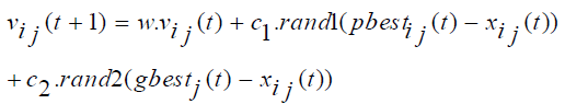
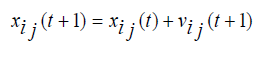
PSO is relatively a new population based search technique for solving numerical optimization problems. It is inspired from the complex social behavior that is shown by the natural species like flock of birds. Each member of swarm called particle associated with a position and a velocity. In the multidimensional search space the particles fly and look for a potential solution. Each particle adjusts its position in the search space frequently according to the flying experience of its own and its neighbors [37]. The movement of each particle is governed by the following two equations (1) and (2), in n-dimensional search space.
 (2.1)
(2.1)
 (2.2)
(2.2)
Where, xi represents the position of the ith particle; vi represents the velocity of the ith particle; pbesti be the previous best particle of the ith particle and gbest is the global best particle found by all particles until now. rand1 and rand2 are two random vector values within (0,1), w represents a inertia weight, c1 and c2 are two learning factors, the value of each velocity vector is compressed within the range (vmax, vmin) to decrease the likelihood of the particle leaving the search space, and t = 1,2,3…, indicates the number of iterations.
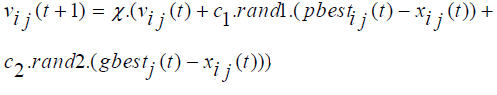
The constriction factor approach of PSO (CPSO) is an important variant of standard PSO, It was proposed by Clerc and Kennedy [38,39]. The velocity of CPSO is updated by the following equation as shown below:
 (2.3)
(2.3)
Where, ? is called a constriction factor, given by equation: 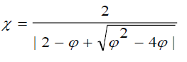 (2.4)
(2.4)
Where,
The CPSO ensures the convergence of the search procedures and be able to generate higher quality solutions than the standard PSO is used in this study.
Functional link neural network
The FLANN architecture was first proposed by Pao et al. [31]. The idea of this model is to apply an expansion function to increases the dimensionality of input vector. Hence the hyper-planes generated provide superior discrimination capability in the input pattern space. The need of hidden layer is removed by applying expansion function thus the learning algorithm become simpler. This model has the benefit to have faster convergence rate and lesser computational cost than MLP structure. The conventional nonlinear functional expansions can be employed in FLANN are trigonometric, power series or Chebyshev type. Majhi et al. illustrates that use of trigonometric function expansion provides superior prediction capability of the model [40]. Therefore, in the present situation, trigonometric expansion is employed. Let us assume each element of the input pattern before expansion is represented as Z(i), 1< i < I where I is the total number of features and each element Z(i) is functionally expanded as Xn (i), 1<n< N, where N is the total number of expanded points for each input element. Let us take, N=5 in this example. The expansion of each input pattern is represented in Figure. 1.The expanded inputs are fed to the single layer neural network and then the network is trained by using training algorithm to obtain the desired output.

Figure 1: Represents the expansion of each input pattern.
Proposed Method
The proposed single layer ANN named as EFLANN with a genetically optimized set of features. It has the potential of generating complex decision regions by nonlinear improvement of hidden units referred to as functional links. Figure. 2. shows the topological structure of the EFLANN. This method is characterized by a set of FLANN with a different subset of features. Let us take the number of original features of the data domain is n and the number of features selected as a chromosome of the genetic population is df, where df ≤ n. The df varies in the genetic population from chromosomes to chromosomes (i.e. 1 ≤ df ≤ n). For simplicity, let us discuss how a single chromosome with df features is working cooperatively for EFLANN.

Figure 2: Topological Structure of the EFLANN.
In this proposed method, the general trigonometric function is used for mapping the df features from low to high dimension. In order to use a function that is very close to the underlying distribution of the data some prior domain knowledge is required. Here five functions are taken out of which four functions are trigonometric and one function is linear (i.e., keeps the original form of the feature value). Within the four trigonometric functions two functions are sine and other two functions are cosine. By using the trigonometric functions the domain is feature values and range is a real number lies between (-1, 1). It can be represented as:
 (4.1)
(4.1)
Where, Domain= {xi1, xi2, ···xidf}, and df represents the number of features. Let us take f1, f2, …., fv be the number of functions that are used to expand each feature value of the pattern. Hence, now each input pattern can be represented as
i = {xi1, xi2, ··· xidf} →{{f1(xi1) , f2(xi1), ··· fv(xi1)}, { f1(xi2) , f2(xi2), ··· fv(xi2)} ···{f1(xidf) , f2(xidf), ··· fv( xidf)} ={{y11,y21, ···yv1}, {y12,y22, ···yv2} ··· {y1df, y2df,··· yvdf}} (4.2)
The weight vector exists between hidden layer and output layer is multiplied with the resultant sets of nonlinear outputs and are supplied to the output neuron as an input. Therefore, the weighted sum is calculated as follows:
 (4.3)
(4.3)
where, i = 1,2···N and m represents the total number of expanded features.
The network has the ability to learn by using PSO training process. The network training needs a set of training data, i.e., a series of input and related output vectors. During the training process, the data is repeatedly presented to the network and weights are adjusted by PSO from time to time till the desired input to output mapping is obtained. Therefore, the estimated output is calculated as follows:
youti(t) = f (sumi), where, i = 1,2···N (4.4)
The error is calculated for ith pattern of training set as
errori(t) = yi(t) – youti(t), where, I = 1,2···N (4.5)
So, the error criterion function is calculated as,
 (4.6)
(4.6)
Here, our objective function is to minimize the error by adjusting weights through CPSO until ε ≤ Er, where ε is very small value.
This process is applied repeatedly for each chromosomes of the GA and subsequently, based on the performance of each chromosome will be assigned with a fitness value. Using this fitness value the usual process of GA is executed until we find some good topology which can achieve an acceptable predictive accuracy.
High level algorithms for EFLANN
The requirements for the near optimal EFLANN architecture and related parameters can be obtained by using both genetic algorithms and Particle Swarm Optimization algorithm for learning. Evolutionary genetic algorithm uses stochastic search and optimization methods. So, GA based on fundamental process, such as reproduction, recombination and mutation. An algorithm of this type starts with a set (population) of estimates (genes), called individuals (chromosomes) encoded properly. For solving the classification task of data mining the fitness of each one is evaluated correctly. The best fit individuals are allowed to make and bear offspring during each iteration of algorithm. The PSO is a population based algorithm used here to update the weights in learning process. During evolutionary process the length of each particle has upper bound n, represents the feature vector. Each cell of the chromosome holds binary value either 0 or 1, where the cell value 1 represents the activation and 0 represents deactivation in functional expansion of individuals. During evolution, each individual measures its effectiveness by the error criterion function that is given in equation (4.6) and then the predictive accuracy is assigned as it corresponding fitness.
Pseudocode for EFLANN
The steps that are followed by EFLANN can be described as follows:
1. Division of Dataset-Divide the dataset into training and testing parts
2. Random Initialization of Individual
3. Each individual Initialize each individual randomly from the domain {0,1}-WHILE (Termination Criterion is Not Met).
4. For the Population
4.1 FOR each sample of the training set
4.2 Mapping of Input Pattern-Map each pattern from low to high dimension by expanding each feature value according to the predefined set of functions.
4.3 Calculation of Weighted Sum-Calculate the weighted sum and feed as an input to the node of the output layer.
4.4 Calculate the Error-Calculate the error and accumulate it.
4.5 Use PSO for Learning-Minimize the error by adjusting weights using PSO.
4.6 Assign the Fitness Value
5. For the Population
5.1 Roulette wheel Selection is performed to obtain the better chromosomes.
6. For the Population Obtained
6.1 Perform recombination
6.2 Mutation
7. While End.
Experimental Studies
The performance of the EFLANN model was evaluated using a set of seven benchmark classification datasets like IRIS, PIMA, BUPA, ECOLI, and Lymphography from the University of California at Irvine (UCI) machine learning repository [41]. For classifying six overlapping vowel classes, we have also taken VOWEL dataset to show the performance of EFLANN [42]. We have used MLP, FLANN with gradient descent learning, RBF and HFLANN results comparison with proposed method. Table 1 summarizes the main characteristics of the databases that have been used in this paper.
| Sl. No. | Name of Dataset | No. of Patterns | No. of Attribute | No. of Classes |
|---|---|---|---|---|
| 1 | IRIS | 150 | 4 | 3 |
| 2 | PIMA | 768 | 8 | 2 |
| 3 | BUPA | 345 | 6 | 2 |
| 4 | ECOLI | 336 | 7 | 8 |
| 5 | LYMPHOGRAPHY | 148 | 18 | 4 |
Table 1: Summary of the datasets used in simulation studies.
Description of the datasets
Let us briefly discuss the datasets, which we have taken for our experimental setup.
IRIS Dataset: This is perhaps the best-known database to be found in the pattern recognition literature. The data set contains 3 classes of 50 instances each, where each class refers to a type of iris plant. One class is linearly separable from the other 2; the latter are NOT linearly separable from each other. The predicted attribute is class of iris plan.
Attribute information:
• Sepal length in cm
• Sepal width in cm
• Petal length in cm
• Petal width in cm
• Class:
o Iris Setosa
o Iris Versicolour
o Iris Virginica
PIMA Indian diabetes dataset
Several constraints were placed on the selection of these instances from a larger database. In particular, all patients here are females at least 21 years old of Pima Indian heritage.
Attribute information:
• Number of times pregnant
• Plasma glucose concentration a 2 hrs in an oral
• Glucose tolerance test
• Diastolic blood pressure (mm Hg)
• Triceps skin fold thickness (mm)
• 2-Hour serum insulin (mu U/ml)
• Body mass index (weight in kg/(height in m)^2)
• Diabetes pedigree function
• Age (years)
• Class variable (0 or 1)
BUPA liver disorders
Data set related to the diagnosis of liver disorders and created by BUPA Medical Research, Ltd.
Attribute information:
• MCV mean corpuscular volume
• Alkphos alkaline phosphatase
• SGPT alanine aminotransferase
• SGOT aspartate aminotransferase
• Gamma glutamyl transpeptidase
• Drinks number of half-pint equivalents of alcoholic beverages drunk per day
• Selector field used to split data into two sets
ECOLI dataset
The reference below describes a predecessor to this dataset and its development.
Reference: "Expert System for Predicting Protein Localization Sites in Gram-Negative Bacteria", Kenta Nakai & Minoru Kanehisa, PROTEINS: Structure, Function, and Genetics 11:95-110, 1991.
Attribute information:
• Sequence Name: Accession number for the SWISSPROT database
• MCG: McGeoch's method for signal sequence recognition.
• GVH: von Heijne's method for signal sequence recognition.
• LIP: von Heijne's Signal Peptidase II consensus sequence score. Binary attribute.
• CHG: Presence of charge on N-terminus of predicted lipoproteins. Binary attribute.
• ALM: Score of the ALOM membrane spanning region prediction program.
• ALM2: Score of ALOM program after excluding putative cleavable signal regions from the sequence.
Lymphography data set
This lymphography domain was obtained from the University Medical Centre, Institute of Oncology, Ljubljana, Yugoslavia. This is one of three domains provided by the Oncology Institute that has repeatedly appeared in the machine learning literature.
Attribute information:
• Class: normal find, metastases, malign lymph, fibrosis
• Lymphatics: normal, arched, deformed, displaced
• Block of affere: no, yes
• Block of lymph. c: no, yes
• Block of lymph. s: no, yes
• By pass: no, yes
• Extravasates: no, yes
• Regeneration of: no, yes
• Early uptake in: no, yes
• Lymph nodes dimin: 0-3
• Lymph nodes enlar: 1-4
• Changes in lymph: bean, oval, round
• Defect in node: no, lacunar, lac. marginal, lac. Central
• Changes in node: no, lacunar, lac. margin, lac. Central
• Changes in stru: no, grainy, drop-like, coarse, diluted, reticular, stripped, faint,
• Special forms: no, chalices, vesicles
• Dislocation of: no, yes
• Exclusion of no: no, yes
• No. of nodes in: 0-9, 10-19, 20-29, 30-39, 40-49, 50-59, 60-69, >=70
Parameter setup
Before evaluating the proposed EFLANN algorithm, we need to set the user defined parameters and protocols related to the dataset. Here we have used two-fold cross validation for all the dataset by randomly dividing the total set of patterns of dataset into two equal parts as dataset1.dat and dataset2.dat. Each of these two sets of dataset was alternatively used either as a training set or a test set [22]. The quality of each individual of dataset is measured by the predictive performance obtained during training. We need to set the optimal values of the following parameters to reduce the local optimality. The parameters we have used are described as follows: Population size: The size of the population designated as |P|=50 is fixed for all the datasets. The number of input features is n. Hence length of the individuals is fixed to n. The probability for crossover is taken as 0.7 and the probability for mutation is 0.02. The total number of iterations we have applied is 1000 for all the datasets. Parameters of PSO for EFLANN training process are set similarly as neural network training with PSO [43]. The MLP uses two hidden layers for all datasets. In each hidden layer P × Q numbers of neurons are taken. Where, P and Q are the number of input neurons and output neurons.
Comparative performance
The predictive performance achieved from proposed EFLANN for the above mentioned datasets were compared with the results obtained from FLANN with gradient descent learning, MLP and RBF results. Table 2. Summarize the comparative average training and test performances of EFLANN with other above mentioned methods.
| Algorithms | ||||||||
|---|---|---|---|---|---|---|---|---|
| Datasets | EFLANN | FLANN | MLP | RBF | ||||
| Training | Testing | Training | Testing | Training | Testing | Training | Testing | |
| IRIS | 98.4710 | 97.4505 | 96.6664 | 96.5662 | 97.1510 | 94.0000 | 38.5000 | 38.5000 |
| PIMA | 80.8220 | 72.6343 | 79.5570 | 72.1355 | 76.6100 | 77.1920 | 77.4740 | 76.0415 |
| BUPA | 77.9830 | 69.3798 | 77.9725 | 69.2800 | 67.5220 | 67.3900 | 71.0125 | 66.9530 |
| ECOLI | 55.3630 | 50.9730 | 49.9625 | 47.3075 | 46.9600 | 45.2650 | 31.1780 | 26.1100 |
| LYMPHOGRAPHY | 98.1590 | 72.7525 | 91.7510 | 74.2800 | 90.2840 | 72.9800 | 85.1365 | 72.2940 |
Table 2: Average comparative performance of EFLANN, FLANN, MLP and RBF.
From Table 2. we can easily verify that in all cases on an average the proposed method EFLANN is giving assuring results in both training and test cases.
Figure.3. shows the percentage of feature selected by the EFLANN in the context of comprehensibility. The datasets are represented by using X-axis and percentage of active bits in the optimal chromosome obtained during the training are represented by using Y-axis.

Figure 3: Represents the percentage of optimal set of selected features in EFLANN.
Predictive accuracy by knowledge incorporation
Let us take n be the total number of features exist in the dataset, F1 and F2 denote the number of feature selected by using the training set 1 and testing set 2 alternatively (Table 3).
| Datasets | N | Predictive Accuracy of Test Set 1 Chromosome |
Predictive Accuracy of Test Set 1 Chromosome |
|---|---|---|---|
| IRIS | 4 | 96.1001 | 97.3260 |
| PIMA | 8 | 71.6525 | 72.9648 |
| BUPA | 6 | 70.5346 | 68.9602 |
| ECOLI | 7 | 54.8939 | 46.9020 |
| LYMPHOGRAPHY | 9 | 79.1374 | 75.9824 |
Table 3: Predictive accuracy of EFLANN by knowledge incorporation with Tr=0.01.,
Notations with Meaning: ?N? denotes the total number of features in the dataset, ?F1?represents the total number of selected features in test set 2. ?F2? represents the total number of selected features in test set 1 and |PA| represents the predictive accuracy.
The fitness of the chromosome related to F1 is
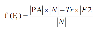 (5.1)
(5.1)
Similarly, the fitness of the chromosome related to F2 is
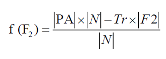 (5.2)
(5.2)
Tr represents the predictive accuracy and tradeoff between two criteria and its value is taken as Tr = 0.01.
Conclusion
In this study, the proposed EFLANN method is used for the task of data mining. It has given importance to the selection of optimal set of features and it has also enhanced the classification accuracy. The classification performance of EFLANN model is promising as demonstrated in experimental studies. Here the architectural complexity is low but, training time is more than FLANN because of feature selection capabilities. Thus implies, this model can be used in medical datasets classification tasks.
References
- Fayyad U, Uthurusamy R. Data mining and knowledge discovery in databases. CommunACM. 1996;39:24-7.
- From data mining to knowledge discovery: An overview. In: FayyadUM, Piatetsky-ShapiroG, Smyth P,editors. Advances in knowledge discovery and data mining. Menlo Park, CA: AAAI Press, 1996, 1-34 p.
- Agrawal R, Imielinski T, Swami A.Database mining: A performance perspective. IEEE Trans. Knowledge Data Eng. 1993;5:914-925.
- James M. Classification algorithms. Wiley, 1985.
- Breiman L, Friedman JH, Olshen RA, et al. Classification and regression learning. Morgan Kaufman, 1984.
- Kriegel HP, Borgwardt KM, Kröger P, et al. Future trends in data mining. Data mining and knowledge discovery, Netherlands: Springer.2007;15(1):87-97.
- Duda RO, Hart PE, Stork DG. Pattern classification. Wiley, New York, 2001.
- GoldbergDE. Genetic algorithms in search, optimization and machine learning. Morgan Kaufmann, 1989.
- Zhang GP. Neural networks for classification: A survey. IEEE T Syst Man Cy C. 2000;30(4):451-61.
- Zhang GP. Avoiding pitfalls in neural network research. IEEE T Syst Man Cy C. 2007;37(1):3-16.
- McCulloch W, Pitts W. A logical calculus of the ideas immanent in nervous activity. Bull Math Biophys. 1943;7:115-33.
- Giles CL, Maxwell T. Learning invariance, and generalization in a higher order neural networks. Appl Optics. 1987;26(23):4972-8.
- Minsky M, Papert S. Perceptrons.The MIT Press, 1969.
- WidrowB, Ho? ME. Adaptive switching circuits. IRE WESCON Convention Record. 1960;96-104.
- Widrow B, Lehr M. 30 years of adaptive neural networks: perceptron, madaline, and back-propagation. ProcIEEE. 1990;78(9):1415-42.
- Wen YU, Li X. Some new results on system identification with dynamic neural networks. IEEE Trans Neural Netw. 2001;12: 412-7.
- Pao YH.Adaptive pattern recognition and neural network. Reading, MA: Addison-Wesley, 1989.
- Young M. The technical writer's handbook. Mill Valley, CA: University Science, 1989.
- Venkatesh SS, Baldi P.Programmed interactions in higher order neural networks: Maximal capacity. J Complexity. 1991;7:316-37.
- Antyomov E, Pecht OY. Modi?ed higher order neural network for invariant pattern recognition. Pattern Recognit Lett. 2005;26:843-51.
- Pao YH, Philips SM. The functional link net learning optimal control. Neuro computing. 1995;9:49-164.
- Misra BB, Dehuri S. Functional link neural network for classi?cation task in data mining. J Computer Sci. 2007;3(12):948-55.
- Mirea L, Marcu T. System identi?cation using functional link neural networks with dynamic structure. 15th Triennial World Congress, Barcelona, Spain, 2002.
- Cass R, Radl B. Adaptive process optimization using functional link networks and evolutionary algorithms. Control Eng Practice. 1996;4(11):1579-84.
- Shin Y, Ghosh J. The pi-sigma networks: An e?cient higher order neural network for pattern classi?cation and function approximation. Proceedings of International Joint Conference on Neural Networks, 1991, p13-18.
- Shin Y, Ghosh J. Computationally e?cient invariant pattern recog- nition with higher order pi-sigma networks. The University of Texas at Austin, Tech. Report,1992.
- Zhu Q, Cai Y, Liu L. A global learning algorithm for a RBF network. Neural Networks 12, 527-540,1999.
- Li M, Tian J, Chen F. Improving multiclass pattern recognition with a co-evolutionary RBFNN. Pattern Recognit Lett.2008;29:392-406,2008.
- Shin Y, Ghosh J. Ridge polynomial networks. IEEE Transact Neural Networks 6(2):610-22.
- Shin Y, Ghosh J. Approximation of multivariate functions using ridge polynomial networks. Proceedings of International Joint Conference on Neural Networks II, 1992;380-5.
- Pao YH, Phillips SM, Sobajic DJ. Neural-net computing and intelligent control systems. Int J Control Syst. 1992;56(2):263-89.
- PatraJC, Pal RN, ChatterjiBN, et al. Identification of nonlinear dynamic systems using functional link artificial neural networks. IEEE Trans Syst Man Cybern B Cybern.1999;29:254-62.
- Dehuri S, Cho SB. Evolutionary optimized features in functional link neural network for classification. Expert Syst Appl. 2010;37:4379-91.
- Dehuri S, Cho SB. A hybrid genetic based functional link artificial neural network with a statistical comparison of classifiers over multiple datasets. Neural Comput Appl. 2010;19:317-28.
- Dehuri S, Roy R, Cho SB, et al. An improved swarm optimized functional link artificial neural network (ISO-FLANN) for classification. j syst software. 2012;85:1333-45.
- Dehuri S, Mishra BB, Cho SB. Genetic feature selection for optimal functional link artificial neural network in classification. IDEAL 2008, LNCS 5326, 2008; 156-163 p.
- Eberhart RC, Kennedy J. A new optimizer using particle swarm theory. Proceedings of the Sixth International Symposium on Micro Machine and Human Science, Nagoya, Japan, 1995, p39-43.
- Clerc M, Kennedy J. The particle swarm explosion, stability and convergence in a multidimensional complex space. IEEE Trans Evol Comput. 2002;6(1):58-73.
- Eberhart R, Shi Y. Comparing inertia weights and constriction factors in particle swarm optimization. Proceedings of the Congress on Evolutionary Computation (CEC2000), pp.84–88,2000.
- Majhi R, Panda G, and Sahoo G. Development and performance evaluation of FLANN based model for forecasting of stock markets.Expert Syst Appl. 2009;36:6800-8.
- Blake CL, Merz CJ. UCI Repository of Machine Learning Databases.
- Pal SK, Majumdar DD. Fuzzy Sets and Decision Making Approaches in Vowel and Speaker Recognition. IEEE Transactions on Systems, Man, and Cybernetics. 1977;7:625-9.
- Carvalho M, Ludermir TB. Hybrid Training of Feed-Forward Neural Networks with Particle Swarm Optimization.In: King I,editors. ICONIP 2006, Part II,LNCS 4233, 2006; 1061-70.
- Hsu CW, Lin CJ. A comparison of methods for multi-class Support Vector Machines. IEEE Trans Neural Netw. 2002;3(2):415-25.