Original Article

, Volume: 6( 3)

• View PDF
• Download PDF

Space System Identification Algorithms

*Correspondence:

Sands T, Department of Mechanical Engineering, Stanford University, USA, Tel: +1-831-656- 3954; E-mail: dr.timsands@stanford.edu

Abstract

System identification algorithms use data to obtain mathematical models of space systems that fits the data, permitting the model to be used to predict and design controls for system behavior beyond the scope of the data. Thus, accurate modeling and characterization of the system equations are very important features of any space mission, especially since guidance and control involves fuel consumption (currently an unreplenishable asset in space). Simple control algorithms begin by using the governing physics expressed in mathematical models for control, but usually more advanced techniques are required to mitigate noise, mismodeled system parameters, of unknown/un-modeled effects, in addition to disturbances. This research article will evaluate several options for mathematical approaches to space identification. Auto-regressive, moving average models will be compared to finite-impulse response filters including relevant iterations such as inclusion of past inputs, uncorrelated output noise, correlated output noise while recursive least squares techniques are compared with exponential forgetting and also compared to extended least squares implementations with iterations to account for posterior residuals. Mean square error is used to help choose system order and the research reveals preferred approaches to readers. The unique contribution of this research is to aid the reader (by direct comparison) ascertain which technique should be used for disparate cases.

Keywords

Exponential forgetting; Posterior residuals; Extended least squares; ARMA; FIR; Transverse filter; Recursive least squares

Introduction

Space system identification applied is often cited to comprise statistical methods to build math models (equations) from given-data, while several useful algorithms are instead calculus-based. The fast Fourier transform [1,2] is ubiquitous for identifying natural frequencies, which are used for a certain class of assumed system models. Which system model should engineers choose? How high must the order of the assumed model be? Goodwin [3] assumed a nonlinear system model and used minimum-variance to estimate system parameters. In particular, Goodwin identified the importance of incorporating white noise (zero-mean with unity covariance) and colored noise. Levin [4] illustrated optimal estimation for impulse response in the presence of noise. Nahi and Wallis [5] illustrated the important applications of system identification to automatic control. Friedlander [6] demonstrated the utility of system identification for adaptive signal processing and Astrom and Wittenmark described the follow-on techniques in their textbook on adaptive control [7]. Slotine [8,9] reveals adaptive control techniques that utilize system math models in their adaptive strategies can often make acceptable system identifiers. Fossen [10] subsequently improved Slotine’s technique with mathematical simplifying problem formulation and Sands [11], [12-17] and Kim [12] developed further improvements to the algorithm based on Fossen’s problem formulation followed by Nakatani [18,19] and Heidlauf-Cooper [20,21], but alas these improvements were not revealed in time for publication in Slotine’s text. Troublingly, Wie [22] elaborated singularities that exists in the control actuation that can exacerbate or defeat the control design as articulated [23-27] and solved by Agrawal [28]. Lastly, Sands [29,30] illustrated ground experimental procedures to perform system identification for initialization of on-orbit methods. Informed by these recent developments, the purpose of this research is to aid (by direct comparison) researchers ascertain which technique should be used for system identification with an underlying motivation of system control.

Materials and Methods

Several methods will be directly compared after a brief explanatory setup for each technique. Transfer functions models are very often a first-stop for mathematical modeling using auto-regressive, moving average assumptions and this article will begin with this technique. Discrete time-shift operators will be introduced that permits the setup methodology to be generalizable to any desired time-indexing for discrete data points. The method is compared to transverse filters using the finite impulse response assumptions and then both techniques are iterated in computer loops to reveal the desired and necessary model-order for a given level of accuracy using the same set of “truth data” for each technique. Next, several modern techniques are implemented on identical data sets and results are plotted on the same graph for easy visual comparison.

Beginning with a truth model (equation 1) to generate noisy outputs measurement time histories, the suitability of various models is investigated to accurately represent the truth data. The goal is to identify the best mathematical model to describe the system that generated the truth data. Next, comparison of various algorithms will be made to evaluate their effectiveness identifying this system when given only the truth data, without any presumed knowledge of the model or its structure,

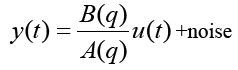(1)

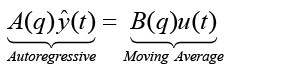
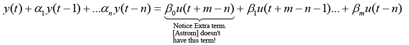
Autoregressive, moving-average model (ARMA), aka “transfer function models”

Using the identical noisy measurement time-history generated by equation 1, polynomial transfer functions with unknown coefficients are used in a least squares algorithm to find the best estimate of the polynomial coefficients. The transfer functions of the system are of the form [7]:

(2)

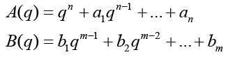(3)

n is the order of the denominator polynomial [A] and m is the order of the numerator [B]. qⁿ implies that time is forward shifted n-times. Note the [A] and [B] matrices are written in terms of forward shift operator ‘q’. Multiply to yield equation 4. Next multiply through by q^-n to express in terms of old data (i.e. you want to avoid an expression that is dependent upon forward shifted…future values) resulting in equation 5 which produces equation 6 implementing the time shift. Multiplyingout to get equation 7, solve for producing equation 8.

(4)

(5)

(6)

(7)

(8)

Implement time shift operations to produce equation 9, e.g.

(9)

Notice a slightly different equivalent development of the form of equation 10 may be multiplied by q^-n shifts time (t-n) producing equation 11.

(10)

(11)

Thus, the degree of the denominator polynomial becomes equation 12, solving for y (t) yields equation 13. The truth model is equation 14 generating the input (random)/output data displayed below in Figure 1. The next task is to estimate the order of the model by comparing mean square errors at model coefficient estimation.

(12)

(13)

(14)

Figure 2 depicts the system input and output. Notice the input control signals are random numbers providing sufficient persistent excitation to estimate all the parameters in the model.

(15)

(16)

In matrix form the truth model (Autoregressive Moving-Average, a.k.a. ARMA) becomes equation 15 and equation 16, thus:

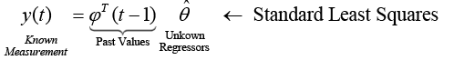
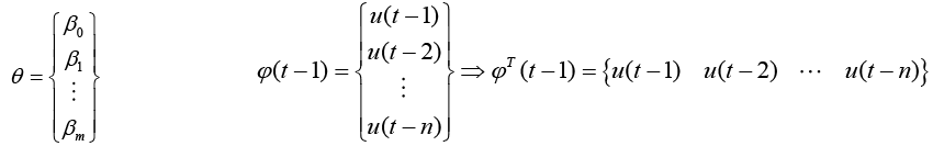
Transverse (FIR) filter

Estimate the model size using a Moving-Average only model first (Transverse or FIR Filter), where we neglect previous outputs (y_i (t-k)) and use the form of standard least squares. The next step is to form the matrices for each time step t per equation 17 where equation 18 minimizes the cost function (equation 19) with a solution in equation 20.

(17)

(18)

to minimize the cost function 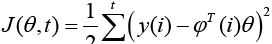(19)

(20)

Iterative results are next displaying mean square error (MSE) for various model orders n^*=n+m’, where n=number of outputs and m’=number of inputs in the assumed model (Figure 1). These results indicate that the mean square error reduces logarithmically as model order increases. Most benefit is gained by the 3-4 order input in the case of transverse (FIR) filter containing inputs only. Certainly nothing beyond 5 seems necessary.

Autoregressive, moving-average model with past inputs

Identical Least Squares analysis was performed using an assumed model that includes past outputs resulting in slightly modified ? and ? matrices, equations 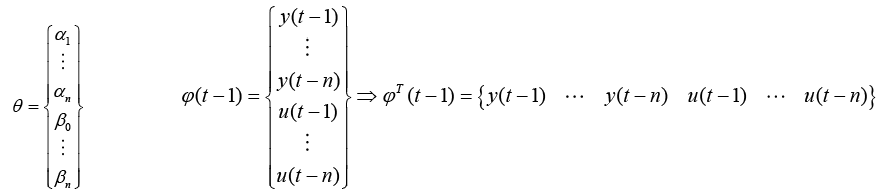21.

(21)

For transfer function models containing inputs and outputs, notice the lowest model order to roughly achieve the minimum on the order of ~10^-20 is n^*=n+m’=3 inputs+3 outputs. Indeed, it appears that we could overstate the model order and achieve slightly improved mean square errors, but the amount of improvement is not worth the risk of overestimating the model order. In this instance, we know that this is the correct order of the model that generated the truth output signal, so we know that we have made a good judgment. Analysis in sections 3.4 and 3.5 of this research article uses 3 y (t) and 3 u (t) terms (Figure 3).

Truth model with uncorrelated output noise

Next, seek to deal with a model that articulates uncorrelated noise seeking the best estimation technique for an assumed model in equation 22.

(22)

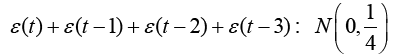
Equation 22 is the new truth model with the addition of an uncorrelated output noise term ε(t)=N (0,1). The truth model is used to generate time history data for 1000 time samples, then recursive least squares is used to estimate the parameters of the assumed model order from section 3.3 (n^*=n+m’=3 inputs+3 outputs). Recursive least squares (RLS) with exponential forgetting (RLS-EF) was also implemented for comparison. Typically, RLS-EF is useful if you believe that you’re plant changes with time. Consider a spacecraft mass model changing as propellant is used during orbit. After considerable orbital maneuvering, it would useful to trigger a reset in the RLS algorithm to determine the new best fit model. The system equation used here does not have model changes, but was implemented nonetheless to evaluate the algorithms’ effectiveness. RLS-EF forgets data as it gets older and older. Without plant changes, intuition says that RLS-EF will not perform as well as RLS. This intuition is confirmed by the following results. λ_EF=0.9 and λ_EF=0.99 (not depicted) were analyzed with inferior performance compared to the other algorithms. λ_EF=0.99 did show marginal improvement over the case of λ_EF=0.9, but not good enough to compare with the other algorithms (Figure 4).

Notice the error plots in Figure 3 and Figure 4, the difference between real coefficients and estimated coefficients reveal our estimate accuracy increases as time progresses. Notice the RLS-EF fluctuates a lot, while the RLS settles to near-zero estimation errors quickly. Consider typical sensors sampling at ~ 40 Hz where 1000 samples are taken in 25 seconds. RLS works pretty quickly on the order of decimal-seconds to rapidly approach a small error value.

Truth model with correlated output noise

Now correlated noise term are considered and RLS with be compared to extended least squares (ELS) and ELS with Posterior Residuals (ELS-PR). Equation 23 is the new truth model (notice the addition of a correlated output noise terms per equation 22).

(23)

(24)

Results and Discussion

Using the exact same time history data y (t), coefficient estimation was performed using extended least squares (ELS). ELS adds the noise terms to the assumed model and attempts to estimate the noise coefficients modifying the least squares variables per equation 25. Lastly, using the exact same time history data y (t), coefficient estimation was performed using extended least squares with Posterior Residuals (ELS-PR). In the ELS-PR algorithm, we calculate an error difference of the output of our best-estimate model and the actual output at that time. Then we declare in the algorithm that all of this error difference is the ε(t) for that time sample.

Notice Figure 5-9 below that ELS-PR is clearly superior. Notice that RLS does okay in the beginning, but is diverging as time progresses. ELS does better than RLS, but still is not handling the correlated noise very well (Recall the uncorrelated error assumption in the Least Squares method). ELS-PR is the best method having the smallest error and generally continuing to converge as time progresses.

It is particularly interesting to note in Figure 8 that the ELS-PR algorithm estimates the errors themselves very poorly, but still performs in a superior manner estimating the actual plant coefficients. Even poor estimates of the errors help improve the estimates of the plant parameters (the things we really care about).

Finally, notice in Figure 9 how much better ELS-PR performs below where the algorithm has been allowed to run for 10,000 time samples. While all 3 methods do a very good job estimating the first control u (t-1) coefficient, only ELS-PR performs well across-the-board. Notice that the other 2 algorithms converge well, but to many incorrect values (displayed by the steady state errors).

Conclusion

This article developed and tested several algorithms used for space system identification and presented direct comparisons of the algorithms on single plots to quickly reveal relative strengths of each approach. Batch least squares was used to reveal that auto-regressive, moving-average (aka transfer functions) filters was superior to finite impulse response (aka transverse) filters at revealing the order of a data set. Next recursive least squares was compared with and without exponential forgetting. Forgetting is useful when the plant equation has a time-varying property, but for non-time varying systems the use of exponential forgetting degrades estimation performance significantly, so minimal forgetting was seen as a wise choice. With that preface, recursive least squares (with and without exponential forgetting) was compared to extended least squares (with and without posterior residuals). Extended least squares performed better than recursive least squares and using posterior residuals with extended least squares proved to be the best choice. Both uncorrelated and correlated noise was investigated. Peculiarly, the extended least squares algorithms poorly estimated the noise coefficients themselves, but inclusion of the error terms for noise in the system model improved estimation of the model equation parameters themselves.

Conflicts of Interest

The authors declare no conflict of interest.

References

1. Annus P, Land R, Min M, et al. Simple Signals for System Identification. Fourier Transform-Signal Processing. In-Tech Publishers. 2012.
2. Heideman M, Johnson D, Burrus C. Gauss and the history of the fast Fourier transform. ASSP Magazine. 1984;1(4):14-21.
3. Goodwin G. Optimal input signals for nonlinear-system identification. Proceedingsof IEEE. 1971;118(7).
4. Levin M. Optimum estimation of impulse response in the presence of noise. IRE Transactions. 1960;CT-7:50-56.
5. Nahi N, Wallis D. Optimal inputs for parameter estimation in dynamic systems with white observation noise. Proceedingsof Joint Auto Control Conference; 1969.
6. Friedlander M. System Identification Techniques for Adaptive Signal Processing. IEEE Transactions on Transactions on Acoustics, Speech and Signal Processing. 1982;30(2).
7. Astrom K, Wittenmark B. Adaptive Control. 2nd ed. Addison Wesley Longman, Massachusetts; 1995.
8. Slotine J, Benedetto M. Hamiltonian adaptive control of spacecraft. IEEE Trans Auto Control. 1990;35(7).
9. Slotine J, Li W. Applied Nonlinear Control. Pearson Publishers, Chapter 8; 1990.
10. Fossen. Comments on Hamiltonian adaptive control of spacecraft. IEEE Trans Auto Control. 1993;38(4).
11. Sands T. Fine Pointing of Military Spacecraft (Ph.D. Dissertation). Naval Postgraduate School, Monterey, USA; 2007.
12. Kim J, Sands T, Agrawal B. Acquisition, Tracking and Pointing Technology Development for Bifocal Relay Mirror Spacecraft. SPIE Proceedings. 2007;6569:656907.
13. Sands T, Lorenz R. Physics-Based Automated Control of Spacecraft. Proc AIAA Space 2009 Conference Exposition. Pasadena, USA; 2009.
14. Sands T. Physics-based control methods. In: Advancements in Spacecraft Systems and Orbit Determination. Rijeka: In-Tech Publishers; 2012:29-54.
15. Sands T. Improved magnetic levitation via online disturbance decoupling. Phys J.2015;1(3): 272-80.
16. Sands T. Nonlinear-adaptive mathematical system identification. Computation. 2017;5(4):47.
17. Sands T. Phase lag elimination at all frequencies for full state estimation of spacecraft attitude. Phys J. 2017;3(1):1-12.
18. Nakatani S, Sands T. Autonomous damage recovery in space. Internat J Auto Control Intell Syst. 2016;2(2):23-36.
19. Nakatani S, Sands T. Simulation of spacecraft damage tolerance and adaptive controls. IEEE Aerospace Proceedings.Big Sky, MT, USA; 2014.
20. Heidlauf P, Cooper M. Nonlinear Lyapunov Control Improved by an Extended Least Squares Adaptive Feed Forward Controller and Enhanced Luenberger Observer. Proceedings of the International Conference and Exhibition on Mechanical & Aerospace Engineering. Las Vegas, USA; 2017.
21. Heidlauf P, Cooper M, Sands T. Controlling chaos – forced van der Pol equation. Mathematics. 2017;5(4):70.
22. Wie B. Robust singularity avoidance in satellite attitude control. U.S. Patent 6039290 A; 2000.
23. Sands T, Kim J, Agrawal B. 2H Singularity-Free Momentum Generation with Non-Redundant Single Gimbaled Control Moment Gyroscopes. Proceedings of 45th IEEE Conference on Decision & Control; 2006.
24. Sands T. Control Moment gyroscope singularity reduction via decoupled control. IEEE SEC Proceedings; 2009.
25. Sands T, Kim J, Agrawal B. Nonredundantsingle-gimbaled control moment gyroscopes. J Gui Control Dyn. 2012;35(2):578-587.
26. Sands T. Experiments in control of rotational mechanics. Internat J Auto Control Intell Syst. 2016;1(2):9-22.
27. Sands T. Singularity minimization, reduction and penetration. J Numer Anal Appl Math. 2016;1(1):6-13.
28. Agrawal B, Kim J, Sands T. Method and apparatus for singularity avoidance for control moment gyroscope (CMG) systems without using null motion. U.S. Patent 9567112 B1. 2017.
29. Sands T. Experimental piezoelectric system identification. J MekhEng Auto. 2017;7(6).
30. Sands T. Experimental sensor characterization. J Space Explor. 2018;7(1).