Original Article
, Volume: 15( 2)Prediction of Drag Coefficient of Spherical Particle Using ANN, ANFIS, Regression and GA Optimization
- *Correspondence:
- Basudeb Munshi , Department of Chemical Engineering, National Institute of Technology Rourkela, Odisha, India, Tel: +916612462265; E-mail: basudebm@gmail.com
Received: May 02, 2017; Accepted: June 15, 2017; Published: June 24, 2017
Citation: Samantaray SK, Sahoo SS, Mohapatra SS et al. Prediction of Drag Coefficient of Spherical Particle Using ANN, ANFIS, Regression and GA Optimization. Int J Chem Sci. 2017;15(2):146.
Abstract
The present work includes the successful prediction of the experimental drag coefficients (CD) as function Reynolds number (Re), collected from the open source literatures by regression analysis method, Artificial intelligence models i.e. artificial neural network (ANN), adaptive Neuro fuzzy interface system (ANFIS) and Genetic Algorithm (GA). A non-linear equation is assumed to relate drag coefficient and Reynolds number and optimized using GA. To confirm the predicted output, twenty-one numbers of inputs are tested and simulated. The comparative study of the prediction models is carried out in terms of the error functions and coefficient of determination. This study has revealed that ANFIS neural model has predicted the desired drag coefficient with minimal error and high coefficient of determination and outperformed the rest prediction models.
Keywords
Drag coefficient; Reynolds number; Artificial neural network (ANN); Adaptive neuro-fuzzy interface system (ANFIS); Regression analysis; Genetic algorithm (GA)
Introduction
Drag coefficient is a very important hydrodynamic parameter for the successful design of industrial processes like clarifiers, thickeners, slurry transporter, cyclone separators, fluidized beds, dust collectors, coal combustors, electrostatic precipitation, and spray drying. Different geometrical shaped particles are present in the process. However, a large volume of research work is available on the drag coefficients of the regular shaped: spherical and cylindrical particles [1-3]. When a solid object is moving through a fluid medium, the aggregate pressure connected on it called pressure drag. The friction drag is a resistive force that appears due to relative motion of the solid body with respect to the fluid medium. The total drag force includes both the pressure drag and friction drag [4]. The movement of an object in fluid medium observes three types of forces, the weight, W of the object acting downward, and the buoyancy¸ FB and the drag force, FD acting upward. The free body diagram at equilibrium is shown in Figure 1.

Figure 1: A free-falling particle under the action of gravity [4].
At equilibrium, the force balance equation can be written as
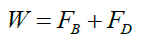 (1)
(1)
Mathematically the drag force can be written as
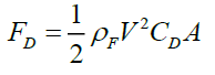 (2) in which V is the terminal velocity of solid particle, ρF is the density of liquid, CD is the drag coefficient. The derived expression of the drag coefficient form Equation (2) is
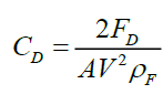 (3)
(3)
where A is the projected area of immersed particle, For spherical particle
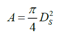 (4)
(4)
in which DS is the diameter of sphere.
The drag coefficient mostly varies with the particle Reynolds number defined as
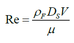 (5)
(5)
where μ is the kinematic viscosity of liquid?
For low Re (creeping flow regime) i.e., Re<0.5, the CD equation is reduced to Stoke’s equation as
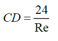 (6)
(6)
Many researchers proposed empirical and semi-empirical equations for CD-Re relation each of which is valid for limited range of Reynolds number [4-7] A summary of those relations is provided in Table1 for the sphere. Similar kind of relations are also available for other type of particle shapes [8-10]. All the references in Table1 also contain their own experimental data which are used in the present work for the prediction purposes.
Since, the proposed empirical and semi-empirical equations have their own range of validations; these cannot be used for the whole range of Reynolds number. Cheng developed unique empirical equations for the drag coefficients with Re which predicted better CD as compared to other emperical relations available in the literature. Cheng used the 408 number of data of [11] which are nothing but the filtered experimental data available in the previous literature, and these data show a very smooth variation of CDwith Re. Therefore, it is quite natural to have high accuracy predicted result by Cheng. Present work felt the requirement of the improved flexible model to predict all the 745 number of the CD – Re data with high accuracy. So, it has become a necessary to develop a high-accuracy predictive model for the drag coefficient, which covers the full range of Re (0 to ∞). The present work has prdicted the drag coefficient with Reynolds number with the help data fiiting, ANN, ANFIS and Genetic Algoithm tools. MATLABTM software is employed for aforesaid analysis.
Data base
In the literature listed in Table 1, the precise data of drag coefficient and Reynolds number are not available; these are reported by the graphs. Hence in order to cover the wide ranges of conditions, experimental drag coefficient data have been picked up from the open literatures listed in Table 1 by using graph digitizer. There are altogether 745 data points.
Prediction Models
Regression analysis
Regression analysis is a well-known curve fitting technique for the nonlinear set of experimental data. It is utilized to describe the relationship between the independent and dependent variables up to the nth order. The main purpose of the regression model is to find a line with the minimum square distance between the experimental data point and line. Henceforth, this model is also called as the least square method [16,17]. A successful regression obtained with some constant terms. It is denoted as E(y/x), where y is the dependent and x is the independent variable. The goodness of predictive model is measured by following statistical terms.
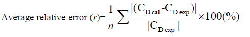 (7)
(7)
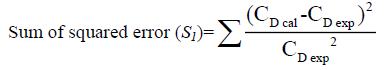 (8)
(8)
 (9)
(9)
The analysis of variance (ANOVA) provides the information about the regression model, which includes R2 and MSE etc., The R2 (coefficient determination) explains the degree of fitting. A perfect regression has R2 close to one and minimum MSE and absolute error percentage. The shape of the CD-Re experimental curve is like exponential shape, which gives the idea for polynomial regression. In this study second order (quadratic) and third order (cubic), regression is carried out.
Artificial neural network
ANN is a numerical model that is based on the human natural nerve framework, and it is used to obtain the solution of complex experimental and scientific problems. Based on the available experimental input and output data, it forecasts the output for any given input. Regardless of this, an ANN model does not require any empirical equation; but adjustment of individual tuning parameter is required to get a fit prediction. Artificial neural networks are comprised of layers. It consists of interconnected nodes called neurons with transfer function. Inputs are introduced to the network through input layer, which sent response to one or more hidden layers, where the weighted sum calculation is carried out using an arrangement of weighted connections. The final network output is obtained through the output layer [18-20]. The basic ANN architecture and the behavior of a neuron are shown in Figure. 2 and 3.

Figure 2: Basic ANN architecture.

Figure 3: Behavior of neuron.
In network, the net input to a neuron is [18]
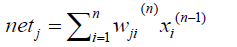 (10)
(10)
where wij is the weight between ith node in (n-1) layer and jth node in (n) layer, and xjn-1 is the output of node j in (n-1) layer.
The weights in BPNN updated as [18]
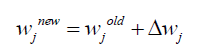 (11)
(11)
Where,
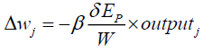 (12)
(12)
Where β, the learning rate parameter lies between 0 and 1. outputj is the output of jth neuron.
The net input to a neuron in any layer is the dot product of the input and the assigned weight factor. In the summation function, the input and weight factors can be associated in different ways before the transfer function. The net result of summation function is transferred to the algorithm based transfer function, where the comparison of summation result with the threshold takes place. There are different types of activation functions available, but the non-linear functions are widely used [19]. The type of activation functions and their ranges are given in Table 2.
| Activation Function | Function | Range of function |
|---|---|---|
| Pure-linear (PURELIN) | f (x) = x | -8, +8 |
| Log-Sigmoid (LOGSIG) | 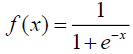 |
0,1 |
| Tan-Sigmoid (TANSIG) |  |
-1,1 |
Table 2: Procedure related characteristics.
Mostly MSE and absolute error percentage are used to evaluate the error [18,20]. MSE is an incremental process, where weights are corrected each time. The adjustment of error is an iterative process, which is done up to the tolerance/goal limit. The basic back propagation network learning is done by the gradient descent algorithm, which helps to minimize the MSE [18,20]. The biggest disadvantage of this algorithm is high time consuming. Aiming to replace the gradient descent algorithm, Levenberg-Marquardt back propagation algorithm (LMBP) is introduced, which incurs the minimum time consumption, high convergence, and low error profile. It is similar to the quasi-Newtonian method, where Hessian matrix is used. The details of the algorithm and weight adjustment of LMBP are described [21]. In this work LMBP algorithm is used for network training and learning.
Adaptive neuro-fuzzy interface system (ANFIS)
The inherent advantages and disadvantages of fuzzy logic and neural network can be disappeared just by combing them. An adaptive neuro-fuzzy interface system (ANFIS) is a hybrid type of the neural network and fuzzy logic approach to predict the data for the nonlinear system of equation. The useful qualitative aspect of fuzzy logic and adaptive aspect of ANN are integrated into ANFIS, which makes the network more reliable, converging and more accurate [22,23]. The learning of network is done with ANN, and the gradient descent algorithm is used in the backpropagation learning of the network. The optimum gradient vector develops the precise modeling of input and output variable for a given set of data [17]. This system is based on a Sugeno system. It can simulate the mapping relation between the input and output data by a hybrid learning to calculate the optimal distribution of the membership functions. It is based worked on the fuzzy “if-then” type rules proposed by Takagi-Sugeno FIS [24]. The used ANFIS network has five layers; each layer includes some nodes represented by node function. The membership functions are tuned using the learning process with a hybrid model, which is a combination of back propagation and least square method [25].
Optimization by using GA
Genetic algorithm (GA) which includes the concept of natural selection and survival of the fittest from natural evolution is a reliable and standard tool to find an optimum solution of a particular problem [26]. It starts with the evolution of population and chromosomes. A stochastic selection procedure is used to find the best chromosomes followed by the crossover and mutation. The best fitness value is evaluated and compared with other best values in population and changed as required. The algorithm stops when either a maximum number of generations is reached, or a satisfactory fitness level is achieved [19]. To develop the correlation of the drag coefficient, C_D with Re using GA toolbox available in MATLABTM, the following nonlinear equation for drag coefficient with Reynolds number is assumed.
 (13)
(13)
The objective function, which is minimized by GA is
 (14)
(14)
Where Y(i) is the experimental drag coefficient and a1(i) is the corresponding Reynolds number. X1, X2, X3 and X4 are the unknown parameters. For GA, to find the optimal solution, the tuning of some population size, selection method and crossover functions, mutation rate, migration, etc. are required. In this regard, the suggested guidelines are available in the literatures [27,28]. The parameters and functions which are used in this study are given in Table 3.
| Options | Value and functions are used |
|---|---|
| Population | - |
| a.Size | 100 |
| b.Creation Function | Feasible Population |
| Fitness Scaling | Rank |
| Selection | Stochastic Uniform |
| Reproduction | - |
| a.Elite Count | 2 |
| b.Crossover Function | 0.8 |
| Crossover | Scattered |
| Mutation | Constraint Dependent |
| Migration | - |
|
a.Forward |
| b.Interval | 20 |
| c.Fraction | 0.2 |
| Stopping Criteria | 100 |
Table 3: Parameter setting for GA optimization.
Results and Discussion
Prediction by regression model
It is observed that third order (cubic) regression predicted outputs have a good agreement with the experimental data in Figure.4. The obtained regression model or equation for drag coefficient-Reynolds number is
 (15)
(15)
Figure 4: Correlation of training patterns in cubic polynomial regression.
The R2 value is obtained as 0.999. The Equation (15) predicted the experimental drag coefficient data very closely at low and medium range of Reynolds number, whereas, a little deviation is observed at higher Reynolds number. The r, S1 and S2 values for this model is given in Tables 4-6. The best fit line equation for cubic polynomial regression is found to be
Y=1.0T+(0.0023) (16)
| Training parameter | Set value |
|---|---|
| Hidden Layer | 1 |
| Maximum number Epoch (No. of Iteration) | 2000 |
| Validation at Fail | 1000 |
| Goal (Tolerance limit) | 1e-03 |
Table 4: Training parameters in ANN.
| Training parameter | Value |
|---|---|
| Type of membership function (MF) | gbell |
| Number of MF | 9 |
| Maximum number of epochs | 100 |
| Error tolerance limit/goal | 1e-03 |
Table 5: Details of the training parameter in ANFIS.
| Prediction model | r | S1 | S2 | R2 |
|---|---|---|---|---|
| ANN | 2.10 | 1.03 | 0.64 | 0.99999 |
| ANFIS | 1.22 | 0.1833 | 0.0354 | 0.99981 |
| GA Optimization | 1.2542 | 0.2610 | 0.0510 | 0.99999 |
| Cubic polynomial regression | 11.58 | 20.28 | 3.10 | 0.99881 |
Table 6: Table of goodness of predictive models.
Where, Y is the predicted output by the regression analysis and T is the experimental output.
Prediction by ANN
Selection of the number of hidden layers, the number of neurons in hidden layer, and the activation function is a challenge for any nonlinear system. It was suggested that for a linear and polynomial system only one layer is sufficient for suitable network training [19]. So, in this work, one hidden layer is chosen. Trial and error method in increasing order is used to find a suitable number of neuron in the hidden layer. It is noticed that after fourteen numbers of neurons in hidden layer, there was no change in MSE in Figure. 5. Hence, one hidden layer with fourteen neurons is adopted for the network training. To find the suitable activation function by keeping the constant number of neurons, several activation functions are considered. The transfer functions, LOGSIG and TANSIG, available in MATLAB are tested, and it is observed that TANSIG produces better result. The training parameters and the trained network for BPNN structure are given in Table 4 and in Figure. 6 respectively.

Figure 5: Variation of MSE as function of number of neurons.

Figure 6: Trained BPNN network structure.
The r, S1 and S2 are computed while comparing the predicted drag coefficients of ANN with the respective experimental data. Arbitrarily twenty-one inputs are selected for training purpose to confirm the predicted output. After 90 epochs, the required MSE is reached as shown in Figure. 7. It is found that the simulated results followed the experimental output trend in Figure. 8. The plotregression command (in MATLABTM) is used for regression analysis, and the value of the coefficient of determination i.e., R2 is obtained as 0.999, which is very close to 1 and it indicates to the development of a perfect correlation between predicted output and experimental output in Figure. 9. The best fit line equation for ANN prediction is

Figure 7: The variation of mean squared error (MSE) with the number of epochs.

Figure 8: Comparison of ANN simulated output with experimental output.

Figure 9: Correlation of training patterns in ANN.
Where Y is the predicted output by ANN.
The calculated r, S1 and S2 with R2 given in Table 6 reveals the good prediction for the drag coefficient by ANN.
Prediction by ANFIS
Generalized bell-shaped membership function (gbell) is used in this study; the shape of gbell MF is shown in Figure. 10. It is found that there is no further improvement in MSE beyond the use of nine numbers of gbell membership functions given in Figure.11. Hence, nine numbers of gbell memberships are used for ANFIS training, which includes nine fuzzy rules in Figure. 12. The ANFIS trained network structure is shown in Figure.13. After training, the same twenty-one input data as taken for ANN are tested. The tested curve follows the experimental output curve in Figure.14. The regression plot for the ANFIS prediction is shown in Figure 15. , where the coefficient of determination R2 is 0.99982 and best fit line as follows
Y=(1.0)T+(0.00048) (18)

Figure 10: gbell membership function of ANFIS.

Figure 11: Variation of MSE with number of membership functions.
Figure 12: Fuzzy rules.

Figure 13: ANFIS network structure.

Figure 14: Comparison of ANFIS testing outputs with experimental outputs.

Figure 15: Correlation of training patterns in ANFIS.
in which Y is the predicted output by ANFIS
Low error profile and high coefficient of determination in Table 6 indicate good prediction capability of ANFIS with the selected parameters given in Table 5.
Optimization GA
In GA method, the fitness and mean fitness are observed in the fitness plot from generation to generations. It is illustrated in Figure. 16 that the fitness value is converging from one generation to another generation. The optimal values of unknown parameters of Equation (13) i.e., X1, X2, X3 and X4 are obtained by minimizing the objective function given in Equation 14, and the developed CD –Re relation by GA is
 (19)
(19)

Figure 16: Convergence pattern in GA.
The coefficient of determination, R2 is found to be 0.998 as shown in Figure. 17. The fit line equation for GA from is
Y=(1.0)T+(0.0018) (20)

Figure 17: Correlation of training patterns in GA optimization.
where Y is the predicted output from Equation 19. The goodness parameters for GA optimization is given in Table 6. Some random input values are tested, and it is observed that the outputs are following the trend line of experimental outputs.
Conclusion
All the predictive models, which are used in this study, have predicted the drag coefficient with excellent accuracy. The relative study of the performance of all the models has revealed that ANFIS model and GA optimization are the best among all the selected models in terms of low error profile and high coefficient of regression. The third order regression model is predicted better in low Reynolds number range and deviated more from the experimental data in higher range of Re. Hence, the cubic regression equation is not suggested. However, the other model i.e., ANN is also equally good, but continuous training is required to obtain the better predicted results. The comparison among the previously existed models and present models (only ANFIS and Equation (19) obtained from GA optimization) is given in Table 7. This table shows the goodness criteria of both ANFIS and Equation (19) are better than the other models. The predicted drag coefficients as function of Reynolds number and experimental data are given in Figure. 18. This work can help to predict the drag coefficient of the sphere at any flow condition. It is expected that this work can be extended to predict the drag coefficients of the other shaped particles.
| Reference | Average relative error, r (%) | Sum of squared relative errors, s1 |
Sum of logarithmic deviations, s2 |
|---|---|---|---|
| Present study (ANFIS) | 1.22 | 0.18 | 0.03 |
| Present study(GA), Equation (19) | 1.25 | 0.26 | 0.0510 |
| Cheng (2009) | 34.96 | 133.03 | 49.25 |
| Brown and Lawler (2003) |
23.66 | 83.33 | 9.90 |
| Clift and Gauvin (1970) |
7.35 | 7.43 | 1.46 |
| Turton and Levenspiel (19860 |
7.28 | 7.07 | 1.39 |
| Flemmer and Banks (1986) | 8.33 | 9.70 | 2.24 |
| Engelund and Hansen (1967) | 87.10 | 1306.241 | 69.51 |
| Khan and Richardson (1987) | 8.21 | 7.61 | 1.56 |
Table 7: Prediction error of different predictive model/equations.

Figure 18: Comparison of predicted outputs vs. experimental measurements as function of input./p>
References
- Almedeij J. Drag coefficient of flow around a sphere: Matching asymptotically the wide trend. Pow Tech. 2008;186:218-23.
- Delleur JW. New results and research needs on sediment movement in urban drainage. J Wat Res Manag. 2001;127:186-93.
- Hvitved-Jacobsen T, Vollertsen J, Tanaka N. Wastewater quality changes during transport in sewers: An integrated aerobic and anaerobic model concept for carbon and sulfur microbial transformations. Wat Sci Tech. 1998;38:257-64.
- Clift R, Grace JR, Weber ME. Bubbles, Drops and particles. New York: Academic Press. 1978.
- Khan AR, Richardson JF. The resistance to motion of a solid sphere in a fluid. Chem Eng Comm. 1987;62:135-50.
- Chhabra RP. Bubbles, drops and particles in non-Newtonian fluids. Boca Raton FL: CRC Press. 1993.
- Hartman M, Yates JG. Free-fall of solid particles through fluids. Chem Comm. 1993;58:961-82.
- Sharma MK, Chhabra RP. An experimental study of free fall of cones in Newtonian and non-Newtonian media: drag coefficient and wall effects. Chem Eng Pro. 1991;30:61-7.
- Unnikrishnan A, Chhabra RP. An experimental study of motion of cylinders in Newtonian fluids: Wall effects and drag coefficient. Can J Chem Eng. 1986;69:729-35.
- Munshi B, Chhabra RP, Ghoshdastidar PS. A numerical study of steady incompressible Newtonian fluid flow over a disk at moderate Reynolds numbers. Can J Chem Eng. 1999;77:113-8.
- Brown PP, Lawler DF. Sphere drag and settling velocity revisited. J Env Eng. 2003;129: 222-31.
- Clift R, Gauvin WH. The motion of particles in turbulent gas streams. Proceeding Chemeca. 1970;70:14-28.
- Flemmer RLC, Banks CL. On the drag coefficient of a sphere. Pow Technol. 198648:217-21.
- Turton R, Levenspiel O. A short note on the drag correlation of spheres. Powder Technology. 1986;47:83-6.
- Engelund F, Hansen E. Monograph on Sediment Transport in Alluvial Streams. Denmark: Hydraulic Lab, Denmark Technical University. 1967.
- Ozel T, Karpat Y. Predictive modeling of surface roughness and tool wear in turning using regression and neural networks. Int J Mach Tool Manufac. 2005;45:112-8.
- Kumanan S, Jesuthanam CP, Ashok Kumar R. Application of multiple regression and adaptive neuro fuzzy inference system for the prediction of surface roughness. Int J Adv Man Technol. 2008;35:778-88.
- Caydas U, Hascalik A. A study on surface roughness in abrasive waterjet machining process using artificial neural networks and regression analysis method. J mat pro technol. 2008;202:574-82.
- Norouzi A, Hamedi M, Adineh VR. Strength modeling and optimizing ultrasonic welded parts of ABS-PMMA using artificial intelligence methods. Int J Adv Man Technol. 2012;61:135-47.
- Davim JP, Gaitondeb VR, Karnikc SR. Investigations into the effect of cutting conditions on surface roughness in turning of free machining steel by ANN models. J mat proc technol. 2008;205:16-23.
- Lin HL, Chou CP. Modeling and optimization of Nd:YAG laser micro-weld process using Taguchi Method and a neural network. International Journal of Advance Manufacturing Technology. 2008;37:513-22.
- Ghamdi KA, Taylan OA. Comparative study on modelling material removal rate by ANFIS and polynomial methods in electrical discharge machining process. Com Ind Eng. 2015;79:27-41.
- Prabhu S, Vinayagam BK. Adaptive neuro fuzzy inference system modelling of multi-objective optimization of electrical discharge machining process using single-wall carbon nanotubes. Aus J Mech Eng. 2015;13:97-117.
- Suganthi XH, Natarajan U, Sathiyamurthy S, et al. Prediction of quality responses in micro-EDM process using an adaptive neuro-fuzzy inference system (ANFIS) model. Int J Adv Manufac Pro. 1991;68:339-47.
- Natarajan U, Palani S, Anandampilai B. Prediction of Surface Roughness in Milling by Machine Vision Using ANFIS. Computer-Aided Design and Applications. 2012;9:269-88.
- Satpathy MP, Moharana BR, Dewangan S, et al. Modeling and optimization of ultrasonic metal welding on dissimilar sheets using fuzzy based genetic algorithm approach. Eng Sci Technol Int J. 2015;18:634-47.
- Goldberg DE. Genetic algorithm in search optimization and machine learning. Boston-MA: Addison-Wesley. 1989.
- Mendi F, Baskal T, Boran K, et al. Optimization of module shaft diameter and rolling bearing for spur gear through genetic algorithm. Expert System Application. 2010;37:8058-64.
