Original Article
, Volume: 6( 1)Photon Probability Control with Experiments
- *Correspondence:
- Solomon BT , Chairman, Xodus One Foundation, 815 N Sherman St., Denver, CO 80203, USA
Tel: 3106663553; E-mail: bts@XodusOneFoundation.org
Received: December 06, 2016; Accepted: March 15, 2017; Published: March 23,2017
Citation: Solomon BT, Beckwith AW. Photon Probability Control with Experiments. J Space Explor. 2017;6(1):116.
Abstract
Quantum theory does not have a mechanism that explains how Nature implements probabilities. Thus, the main objective of this paper is to present new directions for the photonics research for the control of photon localization from probabilistic properties, and another step towards a probability field theory. The expectation is to improve photon collection and loss mitigation. The paper delves into the physics of photon probability control to explain the basis for the 4 new proposed experiments. It is known that photons are not affected by the presence of electric or magnetic fields. Therefore, an alternative question is, can photon probabilities be controlled? Probability control means vectoring and modulation. Vectoring is the control of the direction of localization, and modulation is the control of the distance to localization. This paper proposes a control mechanism by rethinking the foundations of quantum theory, using (i) a modified Schrödinger wave function, (ii) a new structure for particle design, (iii) the existence of subspace (x, y, zand no t), (iv) that all particles consists of a disc of the modified Schrödinger or the probabilistic wave function, orthogonal to the particle’s motion vector and (v) all other particle properties (e.g. electromagnetic wave, charge, mass, etc.) are added to this structure. The shape of the new probabilistic wave function is very close to that of the Schrödinger wave function. It is proposed that probabilities can be controlled by altering the electric and magnetic field densities, as probabilities are function the electric and magnetic fields. Thus, a new formula for the Airy Pattern. Modified Airy Pattern experiments are proposed to confirm these findings. These include measuring the photon’s electric field amplitude, the electric fields in materials, using the Airy Pattern to filter photons by their phase. The new theoretical results confirm that probability is a function of the wavelength. Finally, more than 4 experiments are proposed.
Keywords
Schrödinger wave function; Photon localization photon probability; Airy Pattern; Photon propagation; Electron shell; Probability; Bell’s theorem
Introduction
Quantum theoretic approach
One of the objectives of this paper is to provide an alternative model to the fundamentals of physics, the precursor or prerequisite to quantum theory. It is not about building a better quantum theory. That is unlikely given that over the last 100 years, thousands of expert physicists have checked, double and triple checked this theory as it stands. With an alternative to the foundations of physics one can then falsify (technical usage) quantum theory with three possible outcomes. (i) The foundations of quantum theory are correct and alternative fundamentals are incorrect, resulting in a strong better quantum theory, (ii) The proposed foundations of physics lead to a different and better version of quantum theory or (iii) The interplay between both version, contemporary and proposed foundations, lead to more questions than answers. Given that Nemiroff [1], using Fermi Gamma-Ray Space Telescope photographs of gamma ray burst, showed that quantum foam could not exist, increases the urgency to explore alternatives to the foundations of physics.
Quantum theory describes both mass-based particles and massless particles as exhibiting wave-particle duality. Experimental confirmation of this duality can be found [2] such that (i) the photon particle behavior can be demonstrated by the photoelectric effect (given a work function W) of energy E with photon frequency ν as,
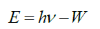 (1)
(1)
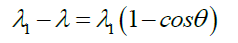
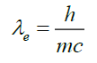
(ii) the electron’s wave behaviour can be described by Compton’s scattering. A photon scattered at angle θ has a longer wavelength λ1 given the electron’s Compton wavelength λe,
 (2)
(2)
 (3)
(3)
And (iii) the de Broglie’s matter wave, that mass matter and massless light satisfy the same energy-momentum and momentum-wavelength (p-λ) relationship,
 (4)
(4)
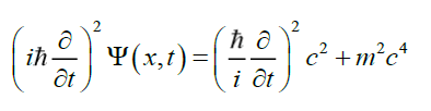
Quantum theory’s wave mechanics is described by the Schrödinger wave equation Ψ(x,t) per
 (5)
(5)
Giving Born’s interpretation of |Ψ|2 as the probability density of finding system at spacetime location (x,t),
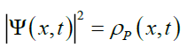 (6)
(6)
Such that the probability density can be moved around, but cannot be created or destroyed in the absence of explicit creative or destructive physical processes. As the physical states in quantum mechanics are linear waves they can be superposed to form other waves using Fourier transforms. And a wave of any kind satisfies the uncertainty relation that for matter waves is the Heisenberg uncertainty principle
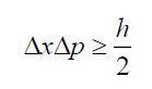 (7)
(7)
Therefore, one notes that quantum theory is essentially a wave theory used to describe particle behavior, with all non-wave properties (probabilities for example) described in terms of this wave nature. Photons in particular are also modelled using wave equations known as Bessel functions. As Roychoudhuri [3] proposed, “We need to embark anew on comprehensive foundational studies about generation, propagation, and detection of EM waves across the entire spectrum. Huygens- Fresnel’s wave picture and Einstein-Dirac’s indivisible quanta represent one of the strongest unresolved issues in physics.
While the authors agree with his premise for the need for foundational studies, the authors differ in approach. Solomon and Beckwith [4] laid the ground work required to model photon behaviour in terms of probabilities instead of wave equations or Bessel functions. This paper adds to that work [4].
How is it possible to derive an alternative to wave equations? In Operations Research, there is a class of mathematic search techniques, mathematical programming, that have a unique property known as Primal-Dual formulations. Mathematical programming consists of an objective function that is matrix row, a matrix of constraints whose inequalities form a matrix column of boundary conditions, known as the Primal problem. The Dual problem exists when the constraint matrix rows and columns are swapped, and concurrently, the objective function is swapped with the boundary conditions. It turns out that the solution to the Primal formulation is identical to the solution of the Dual formulation. That is, two apparently different formulations of the same problem have identical solutions.
The point spread function (PSF), here termed Airy Pattern (not Airy Disc), of photons projected through a pin hole to a screen, is the basis of this deconstruction. However, the modern definition of this type of PSF is a Bessel function expressed only in terms of wave functions and therefore not suitable for the proposed deconstruction, as the Bessel functions have entirely removed the photon’s probabilistic behaviour. The wave Bessel functions can be considered the Primal formulation. To determine the probabilistic behaviour, the Dual formulation, one has to go back to the older formulation (Appendix B) of the Airy Pattern. As proof that this Dual formulation exists, the probabilistic Dual formulation should give identical results to the Primal Bessel formulation. That is, if the primal formulation wave equations can describe probabilities, then the Dual formulation probability density should be able to describe wave behaviours.
Further, there is in physics research, what is known as the pilot model [5], which has a specific re-interpretation of probability, and not just on the basis of wave interference. Quoting [6].
The Copenhagen interpretation is essentially the assertion that in the quantum realm, there is no description deeper than the statistical one. When a measurement is made on a quantum particle, and the wave form collapses, the determinate state that the particle assumes is totally random. According to the Copenhagen interpretation, the statistics don’t just describe the reality; they are the reality.
The research in this paper is to determine another layer of statistical inference, as an alternative to the Copenhagen interpretation, and that is what the offered aim of this paper is.
Why rethink photon probabilities?
In 2015, Steinhardt and Esftathiou [7] stated that the Planck Space Telescope data shows that the Universe is simpler than had been thought and that both string and quantum theories require revisions. To add to this debate, in 2012 using NASA's Fermi Gamma-ray Space Telescope photographs of gamma ray burst, Nemiroff [1] showed that quantum foam could not exist.
Solomon [8-13] proposed that contemporary physics can be categorized into three types of particles, inelastic and point-like (quantum theory), tensile (strings) and compressive. Assuming that particles were compressive Solomon [8-12] proved that a new equation for gravitational acceleration (1) that does not require a prior knowledge of the amount gravitating mass.
 (8)
(8)
Where τ is the spatial gradient of the time dilation transformation or change in time dilation transformation divided by that distance, and noting that the time dilation transformation is the ratio of tv/t0 per Lorentz-FitzGerald transformations (LFT) or (9), and Newtonian Gravitational Transformations (NGT)or (10). Thus, Solomon’s g=τc2 provides a mathematical solution to Hooft’s [14] assertion that “absence of matter no longer guarantees local flatness”.
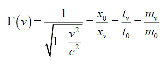 (9)
(9)
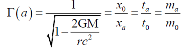 (10)
(10)
The existence of (8) raises substantial doubts about the validity of string theories as strings are based on the opposite axiom that particles are tensile. Further, strings contradict Lorentz-FitzGerald transformations (LFT).
Therefore, pursuing Steinhardt and Esftathiou’s [7] need for a different approach to the physics, there are fundamental questions that need to be answered, (i) How are probabilities implemented in Nature? and (ii) Can these probabilities be controlled? The objective of this paper is to present photon probability functions as an alternative to Bessel functions, to model photon behaviour.
Roychoudhuri [3] summarizes that there are two types of photon models, (i) Huygens-Fresnel’s wave and (ii) the Einstein-Dirac’s indivisible quanta. As Roychoudhuri [3] states, the definition of a photon by quantum electrodynamics is something like an indivisible packet of energy but represented by a Fourier monochromatic mode of the vacuum which is problematic, for the following reasons:
• Such individual photons cannot be localized in space and time.
• An infinitely long Fourier mode violates the principle of conservation of energy.
• Superposition of many Fourier frequencies creating a space-finite pulse in free-space to model pulsed light is an invalid conjecture because waves cannot interact and regroup their energies in the absence of interacting materials.
• It assigns rich properties to “vacuum” and yet relativity and quantum physics do not explicitly recognize space as a real physical medium.
• The quantum photon’s indivisibility directly contradicts the immensely successful HF diffraction theory.
Using Roychoudhuri’s critique as a basis for comparison, one can state that this paper proposes a third model derived from the Airy Pattern, an infinitely thin disc whose plane (x-y axes) is orthogonal to the photon’s motion vector along the z-axis, that is not infinite (per ii), and based on a “richer” (per iv) property of spacetime, one that involves deformable spacetime(x, y, z, t) and deformable subspace (x, y, z).
Probabilistic Wave Function Ψp Derivation from the Airy Pattern
Quoting Richard Feynman1 regarding the Schrödinger wave function, “When Schrödinger first wrote it down, he gave a kind of derivation based on some heuristic arguments and some brilliant intuitive guesses. Some of the arguments he used were even false, but that does not matter; the only important thing is that the ultimate equation gives a correct description of nature.”
Therefore, since the Schrödinger wave function works, is it possible to derive the Schrödinger wave function from the empirical data? The derivation below gives a wave function, Probabilistic Wave Function ψP, that is very similar to Schrödinger’s.
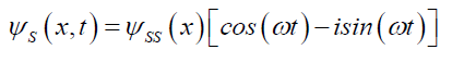
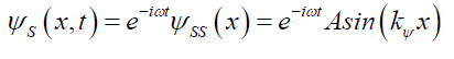
Excerpted from [15] the following details how the Probabilistic Wave Function ψP was derived from the Airy PatternψA. The necessary assumption is that the particle’s wave function (Schrödinger or otherwise) can be determined from its projection, the Airy Pattern, on an opaque screen. That the two, the particle’s wave function and the Airy Pattern, are related by a cause (particle’s wave function) and an effect (the Airy Pattern). Schrödinger’s2, ΨS(11) with their respectively solutions ψ and ψS and quantum mechanical spatial solution ψSS,
 (11)
(11)
 (12)
(12)
 (13)
(13)
 (14)
(14)
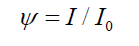
Where A is the maximum amplitude, A sin (kΨx) is the amplitude between nodes at distance x, and ω is angular frequency of this standing wave. Figure. 1. (red solid line) shows the solution ψ (12) to the Probabilistic Wave Function Ψ,

Figure 1: Probabilistic wave solution ψ (solid red) and its 2 components, χ (dashed grey) and φ (dot-dash green).
 (15)
(15)
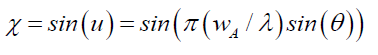
This probabilistic wave solution ψ can be deconstructed from 2 components. The first, is the wave term in spacetime, the space wave χ (Figure. 1. dotted grey line), (13)
 (16)
(16)
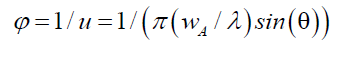
And the second is the envelope probability density function φ (Figure. 1. dashed green line) of un-normalized probabilities from the u function of (14), as follows,
 (17)
(17)
Such that,
 (18)
(18)
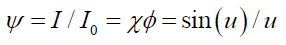
In effect, the wave space wave χ (16), weights the probability envelope probability density function φ (17), to produce the probabilistic wave solution ψ(18). This weighting is equivalent to the space wave χ casting a shadow on the envelope probability density function φ and upper bounds the probabilistic wave solution ψ in a consistent mathematical manner.
Space wave χ (Figure. 1. dotted grey line) has a constant amplitude (maximum of I/I0=1) and damped period. This is because the space wave χ wavelength λχ increases as the radial distance rA increases. Compare (12) with damped oscillations3 (19).
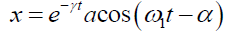 (19)
(19)
Where γ is the damping coefficient, a amplitude, α is phase, and ω1 is related to damped oscillations.
Clearly, the Schrödinger’s wave function solution ΨS (12) is a damped oscillation that is phase shifted. Replacing the inverse function envelope probability density function φ with an equivalent exponential4 term (20), and the time t variable with radial distance rs gives (21), a damped oscillation version of ψ.
 (20)
(20)
 (21)
(21)
Both the inverse (17) and the exponential (20) forms of the envelope probability density function φ term appear similar. The exponential term (20) is at best a good approximation5 but not a perfect fit. Therefore, neither the space wave χ nor the probabilistic wave solution ψ are damped spatial oscillations.
However, both the space wave χ and the probabilistic wave solution ψ have damped spatial periods, as determined by (16). (16) shows that the space wave χ, is constant when θ is constant, that is, where the ratio of rA to dA is constant,
 (22)
(22)
 (23)
(23)
As a function of θ, (22) confirms that the space wave χ, is not a time varying standing wave function, kθ(wA/λ)π represents the phase shift of these spatial oscillations, and spacetime disturbance χ is the outward projection of the particle’s own wave function. By (16) and (22), (24) confirms that the envelope probability density function φ is a spatial geometric structure whose probability decreases with the particle’s wavelength λ.
 (24)
(24)
That is, the higher the energy of the particle, the smaller the space wave χ, and lower the probability of particle localization within this smaller geometry. Therefore, the space wave χ, the envelope probability density function φ and thus, the probabilistic wave solution ψ are derived from a common mechanism for all particles.
It is proposed that the shape of the particle’s probabilistic wave solution ψp can be reconstructed from its space wave χp and its envelope probability density function φp. Assuming the particle occupies some space, extrapolating back (along the zaxis) to the center of the particle, dA=0 would give,
 (25)
(25)
Along both the x- and y-axis, given x the distance from the center of the particle, the aperture wA=2x. Given kΨ (13), by (23) particle’s space wave χp is,
 (26)
(26)
From (24) the particle’s envelope probability density function φp is,
 (27)
(27)
And from (16) the particle’s probabilistic wave solution ψp is,
 (28)
(28)
The particle’s probabilistic wave solution ψp (28) explains how Airy Pattern and interference patterns are produced. The particle’s envelope probability density function φp is the maximum probability amplitude and its space wave χp determines the oscillations along the x- and y-axes. Note also, that the particle’s space wave χp (26) is not period damped like that of the interference patterns space wave χ (23). This affirms that the latter (23) is a projection of the former (26).
Since (28) is non integrable, it will not be easily to reverse engineer a Schrödinger-type wave function, if one exists. A non integrable probabilistic wave solution ψ (28) would concur with the thesis that this wave function is an orthogonal displacement in spacetime which is not motion.
Therefore, along the z-axis by (22), as θ→0
 (29)
(29)
And as
 (30)
(30)
 (31)
(31)
However, θ→0
 (32)
(32)
Equation (28) describes the particle’s wave function Ψp=ψp in both the x- and y-axes while the z-axis function (32) is a constant 1. It shows that, the particle wave function along the z-axis is not a function of this distance, and thus the wave function is orthogonal to the particle’s motion. The particle’s intensity shape is symmetrical conic-like disc in the plane orthogonal to motion, but its physical shape is an infinitely thin disc. This is a structure that would be consistent at any velocity vp<c and vp=c.
The basic particle can be described, Solomon [15], as umbrella shaped, consisting of a wave function disc and probability disc that are orthogonal to its motion vector. Therefore, there are 5 parts to a basic particle, i) motion vector, ii) space wave χp disc (26), iii) probabilistic envelope probability density function φp disc (27) that iv) combine to form the probabilistic wave solution ψp disc (28) and v) the projected probabilistic wave solution ψ disc (18) that results in the diffraction patterns. All other properties (e.g. mass, electric field and magnetic field) are added to this structure. The utility of this umbrella shape is that “orbiting” electrons with motion vectors pointing to the center of the nucleus will not produce synchrotron radiation, and therefore, by inference do produce photon emissions when not.
Solving for Airy Pattern Probability With [1/(Kλr)] Sin(Kλr)
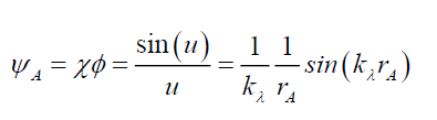
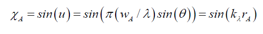
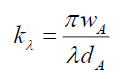
The objective of this section is to solve the range of value for which the Airy Pattern’s wave function ψp exists. Note, the point spread function (PSF), here termed Airy Pattern, of the photons projected through a pin hole to a screen, is the basis of this deconstruction. However, the modern definition of this type of PSF is a Bessel function expressed only in terms of wave functions and therefore not suitable for the proposed deconstruction. Therefore, reverting to the old definition of the Airy Pattern’s wave function ψA (33) and its corresponding space wave χA (34), and envelope probability density function φA (35), given the pinhole aperture diameter wA, the distance between pin hole and screen dA and angular displacement θ from pinhole a radial position rA on the screen,
 (33)
(33)
 (34)
(34)
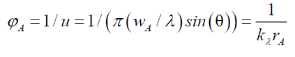 (35)
(35)
Where, for small θ,
 (36)
(36)
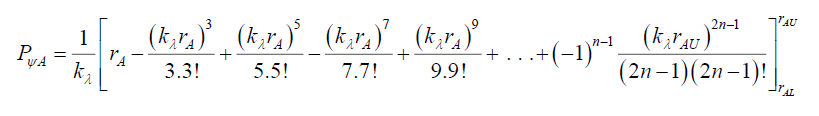
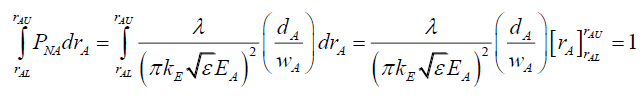
For a radial path, the Airy Pattern ψA (33) along a radius rA as a probability density function of photons arriving at the screen a distance dA from the pin hole of with wA, gives, the total probability density PψA of,
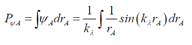 (37)
(37)
To Determine the Lower Bound rAL
For r≠0, and r>0 gives,
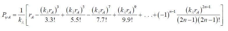 (38)
(38)
Because the series has to converge very quickly, kλ is very much less than 1, and numerical testing (Table 1) shows,
| Visible Light Spectrum (mm) | kλ | PψA | rψ | PψA/rψ | |
|---|---|---|---|---|---|
| Violet | 400 | 5.09E-10 | 1.07E-02 | 1.07E-02 | 1.00E+00 |
| Indigo | 445 | 5.67E-10 | 1.19E-02 | 1.19E-02 | 1.00E+00 |
| Blue | 475 | 6.05E-10 | 1.27E-02 | 1.27E-02 | 1.00E+00 |
| Green | 510 | 6.49E-10 | 1.36E-02 | 1.36E-02 | 1.00E+00 |
| Yellow | 570 | 7.26E-10 | 1.52E-02 | 1.52E-02 | 1.00E+00 |
| Orange | 590 | 7.51E-10 | 1.58E-02 | 1.58E-02 | 1.00E+00 |
| Red | 650 | 8.28E-10 | 1.74E-02 | 1.74E-02 | 1.00E+00 |
Table 1: Airy pattern probability rAL calculations.
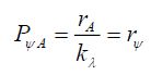 (39)
(39)
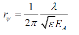
Where, (see Appendix D, deriving rψ, on how rψ was arrived at),
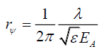 (40)
(40)
That is, rA is lower bound rAL,
 (41)
(41)
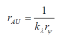
To determine the upper bound rAU
For rA=rAL to rA=rAU gives,
 (42)
(42)
Because the series converges very quickly,
 (43)
(43)
As rAL≈0.
 (44)
(44)
Therefore, the Airy Pattern probability PA along a radius rA,
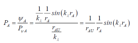 (45)
(45)
Since the maximum probability must be 1 for any value of rA, when rA=rALfrom (45) the coefficient of the sine function be 1,
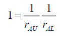 (46)
(46)
Therefore,
 (47)
(47)
That is,
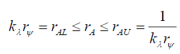 (48)
(48)
Therefore, the Airy Pattern probability PA along a radius rA,
 (49)
(49)
Therefore, the question, why isn’t there a dark spot at rA=rAL? It is for two reasons, (i) at certain distances dA this is observable, and (ii) photon probabilities PN(θ,r) cause this dark spot to be smudged.
Solving for Photon Probability With [1/(kψr)] Sin(kψr)
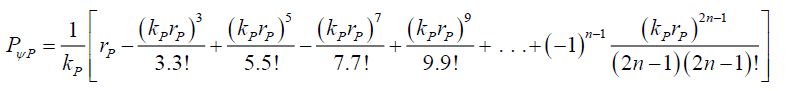
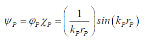
The photon’s Probabilistic Wave Function ψP (50) can be deconstructed into the space wave χP(51), and the envelope probability density function φP(52) with the total probability density PψP because it is derived from the Airy Pattern, some of the properties of the Airy Pattern function ψP are borrowed from Solving for Airy Pattern Probability with [1/(kλr)] sin(kλr). Therefore, what needs to be determined first is kP. and rψP
 (50)
(50)
 (51)
(51)
 (52)
(52)
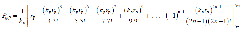
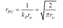
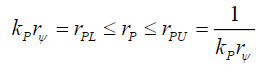
To determine the lower bound rPU
For rP ≥ rPL gives,
 (53)
(53)
Because the series converges very quickly as kPrP, and assuming that the form of (39) is still valid
 (54)
(54)
Where the total probability density is PψP or,
 (55)
(55)
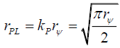
To determine the upper bound rPU
 (56)
(56)
Because the series converges very quickly as kPrP, and assuming that the form of (39) is still valid, and as rPL≈0
 (57)
(57)
Therefore, the photon probability PP along a radius rP,
 (58)
(58)
Since the maximum probability must be 1 for any value of rP, when rP=rPLfrom (58) the coefficient of the sine function be 1,
 (59)
(59)
Therefore,
 (60)
(60)
That is,
 (61)
(61)
From (58) a necessary condition for maximum probability to be 1 when rP=rPL is that the sine function must be 1, too. Therefore,
 (62)
(62)
Or, from (12),
 (63)
(63)
And,
 (64)
(64)
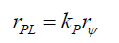
Or,
 (65)
(65)
 (66)
(66)
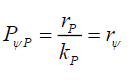
The total probability density DψP of the photon disc is the radial probability density PψP rotated from 0 to 2π radians. By (61) and (67),
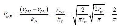 (67)
(67)
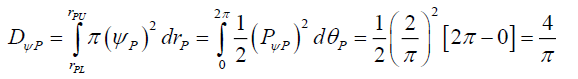 (68)
(68)
That is, the total photon probability density PψP along any orthogonal radius is a constant 2/π, and the total disc probability density DψP is also a constant 4/π.
Airy Pattern probability
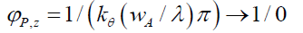
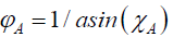
From the perspective of probability control, there are some challenges that need to be solved. First challenge is, how to control probability of localization? From (35) it is clear that the probabilistic envelope function φA is a function of photon frequency ν and photon constant kA or,
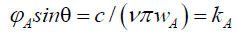 (69)
(69)
That is, the probabilistic envelope function φA is an inverse function of angle θ from axis or given a pinhole to opaque distance dA and the orthogonal radius rA on the opaque screen,
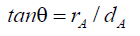 (70)
(70)
From (34) (71)
Or
 (73)
(73)
Or it is the space wave χA oscillations that causes the changes in the probabilistic envelope function φA. Without experimental evidence, it is difficult to propose correctly how the space wave χA can be altered. However, some direction can be inferred as to how to conduct these experiments. Since it is the [15] electromagnetic wavelength λem that determines the space wave χA wavelength λχ (or the other way around),
 (73)
(73)
Therefore, electromagnetic fields can be used to alter the space wave χA and therefore, alter the probabilistic envelope function φA. By rewriting (69) in terms of photon energy hν,
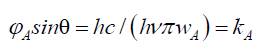 (74)
(74)
One notes as photon energy increases, its wavelength decreases and by (72) so does the space wave χA wavelength λχ. This causes the normalized probabilities to occupy a smaller space.
Another approach would be derived from Figure. 1. [15], which shows that the peak intensity (solid red) function is capped by the probabilistic envelope function φAand oscillates with the space wave χA. Assuming field commutative symmetry [10,13] then the presence of any two of the fields would result in the third.
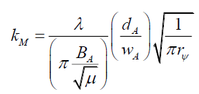
Thus by (74) peak electric or magnetic field strength is capped by probabilistic envelope function φA. To keep it simple, if the space wave χA was flat then, the electric and magnetic field strength would be (at least approximately) linearly dependent on the envelope function φA. Therefore, by field commutative symmetry the electric or magnetic fields would alter probabilities,
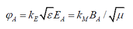 (75)
(75)
Where kE and kM are the respective electric and magnetic field constants, and the utility of using √ε and √μ-1 will become evident.
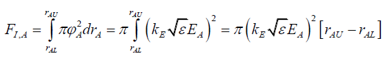
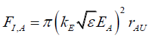
For the Airy Pattern formed by the rotation of the radial path about the axis of the pin hole, the total spatial probability distribution must sum to 1, at or in the field of interaction FI irrespective of this field’s shape. This field of interaction FI is determined on a case by case basis. It is the area A of the plane as in the screen for Airy Pattern experiments (76) and the volume V of space (77) for 3-dimensional chemical reactions.
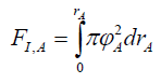 (76)
(76)
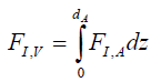 (77)
(77)
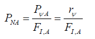
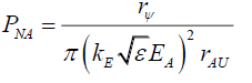
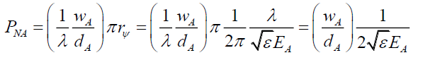
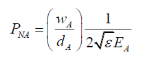
Where rA is from 0 or from the axis of propagation through the aperture, to the radial distance rAU on the screen. The normalized probability PNA of a photon localizing at the disc with radial coordinates (θ,r) on a screen a distance dA, using the Probabilistic Wave Function ψA(θ,r) PψA, it would take the form, from (39),
 (78)
(78)
Where,
 (79)
(79)
 (80)
(80)
Field commutative symmetry is borrowed from (http://mathworld.wolfram.com/) the mathematical definition of commutative, where under certain conditions give the same result independently of the order of the elements. For example addition, multiplication, algebra, diagrams, monoids and rings are or can be commutative. Thus, with respect to fields, field commutative symmetry is defined as the interchangeability of orthogonal fields such that when two orthogonal fields are required to produce a third orthogonal field, it does not matter which two is initiated, the third field produced is the remaining field, when all necessary factors are present. For example, a moving (velocity v is present) electric field E would evidence a magnetic field B. Similarly moving (velocity v is present) magnetic field B would evidence an electric field E. And an oscillating electromagnetic field would evidence velocity. Therefore, it does not matter the order of the fields selected, all three will be present. Thus, the velocity-electric-magnetic field example proves that Nature demonstrates field commutative symmetry. This field commutative symmetry could be applied in other relationships.
By (48),
 (81)
(81)
Since, rAL≈0,
 (82)
(82)
 (83)
(83)
From (75) the lower rAL and upper rAU bounds are given by,
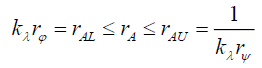 (84)
(84)
The lower bound rAL implies that intensity cannot reach infinity.
 (85)
(85)
From (36)
 (86)
(86)
That is, since,
• As electric field, maximum amplitude EA increases, probability decreases and the photon is less likely to localize. For optical fiber laser amplifiersi, the pump wavelength supplies energy to boost the signal wavelength energy and much work is required to explore this avenue further.
• As wavelength λ decreases probability decreases and the photon is less likely to localize, and the photon is more 1http://www.feynmanlectures.caltech.edu/III_16.html likely to pass through an opaque screen or more likely to behave like a particle rather than a wave.
To determine kE, consider that the total probability along any radius rA=1, assuming that kE is a constant,
 (87)
(87)
By (82), and since rAL≈0,
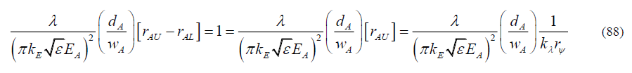
Or,
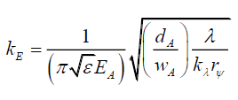 (89)
(89)
By (41),
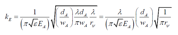 (90)
(90)
Similarly,
 (91)
(91)
Therefore, by (86), (90) can be rewritten as, (Appendix A, Numerical Modeling Tables),
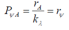
And by (52),
 (93)
(93)
Similarly,
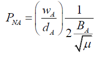 (94)
(94)
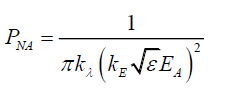
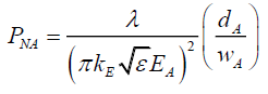
That is, the probability of localizing to form an Airy Pattern is
• An inverse function of the electric EA or magnetic BA field amplitude.
• A function of the ratio of the pinhole width wA and distance from screen dA.
• Not dependent on the photon wavelength λ.
• The surprising inference is that while photon probability is altered by its electric EA and magnetic BA field strength (93) and (94), the photon energy EP=hν is not. Therefore, one infers that the photon energy is derived from the oscillation of the transverse wave’s non-zero electric EA and magnetic BA fields amplitudes and not their specific amplitudes.
• This raises the question, is the observed oscillation due to the phase and orientation of the electromagnetic wave arriving at the pinhole? This is a very likely mechanism and could be an example of the observer altering the observation with a pin hole. To explore this one first has to add the effect of external electric field due to the pin hole.
Explaining the Airy Pattern Intensity
To answer why the Airy Pattern intensity in non-linear (38) while the photon probability on this Airy Pattern is a constant (93) and (94), this analysis deconstructs the photon into it individual parts, amplitudes EA and BA and phase α.
A pin hole, after all, is a circular electric field of magnitude EH along any radius, formed by electron shells of the material surrounding the pin hole. Therefore, from (93), the photon probability PEA in the presence of an external electric field EH is,
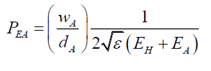 (95)
(95)
To evaluate, in the presence of the pin hole external electric field EH, how photon phase α arrival alters probability PNA, the varying electric field amplitude EE was set to EE such that,
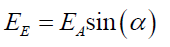 (96)
(96)
And the phase altered probability PαA of an individual photon using (95) is given by, (See Appendix A, Numerical Modeling Tables),
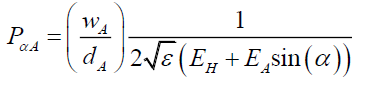
Therefore, logically,
• A minimum interference with the pin hole’s electric field EH occurs when the phase α=0°, and sin(α)=0. The photon passes straight through the pin hole as if the pin hole did not exist as its electric field is zero. Therefore, rA=rAL.
• This suggests that the more interference with the pin hole the greater the phase of the electric field.
• Therefore, one could propose that α=90°, when the deflection is maximum, or rA=rAU (Figure 2).
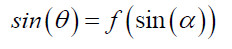
• For monochromatic photons, the radial deflection θ, on the Airy Pattern is monotonic with respect to α,

Figure 2: Photon probability projected on to the airy pattern.
 (98)
(98)
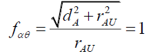
Proposing a monotonic function (99) to determine the function fαθ,
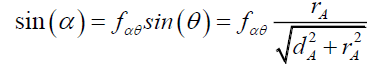 (99)
(99)
When α=90 , and the upper bound radial displacement rAU on the Airy Pattern (Figure 2), gives,
 (100)
(100)
 (101)
(101)
Or,
 (102)
(102)
Substituting back into (99) and resolving for rA gives,
 (103)
(103)
Since rAU >> dA,
 (104)
(104)
And,
 (105)
(105)
Or,
 (106)
(106)
or,
 (107)
(107)
That is, the radial θ spread is entirely due to the photon phase α arrivals, and (97) is the correct phase altered probability PαA of an individual photon. (97) also, accounts for the non-linear decrease in intensity along the radius, i.e. it explains the coefficient term space wave χA (34) in the Airy Pattern ψA (33). If (107) can be experimentally verified, it can significantly reduce diffraction in optical instruments by using photons of a single phase (e.g. lasers), and is a means to filtering photons by their phase.
The Airy Pattern ψA (33) probabilities display the decreasing oscillations. Controlling for phase α arrivals shows that probabilities are altered by phase α arrival and are evidenced as decreasing strength of the probabilities along a radius rA.
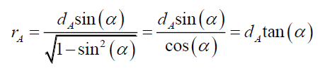
Just as the amplitude of the electric field EA at the pin hole affects the radial displacement θ, the amplitude of this electric field EA will alter the probability of localization at the radial distance rA. That is, if the photon travels along the hypotenuse formed by dA and rA, the phase of the photon βA at arrival is what needs to be determined. The number of cycle nA along the hypotenuse is given by,
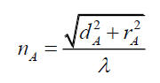 (108)
(108)
Adding the phase α start of the photon at the pin hole, the phase γA along the hypotenuse is given by,
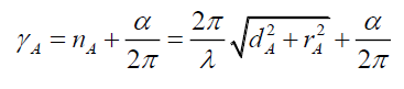 (109)
(109)
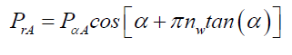
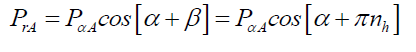
Therefore, phase γA modified probability PβA is a cosine function as intensity is a maximum when rA=0 and this term must range between 0 and ± 1.
 (110)
(110)
Testing numerically, shows that (110) is not the correct behavior as this gives what appears to be random scramble of photons compared to the Airy Pattern. Other variations of (110) were tested with no joy. This suggests that the photon does not travel along the hypotenuse, and that the Airy Pattern ψA (33) oscillations are a much more sophisticated phenomenon (Figure. 3).

Figure 3: Airy Disc α and Probability of cos(α+β).
Since probabilities are a function of the photon’s electric field maximum amplitude EA (95) and per the proposed experiment in §11, what if this electric field strength dilutes with the radial distance rA? A possible dilution model is the total probability PαA over a disc formed by rAL should be equal to the total probability PrA over a disc formed by rA, thus,
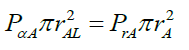 (111)
(111)
Or,
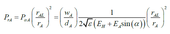 (112)
(112)
This, too, is not how Nature works. Reviewing (33) suggests that only the displacement rA along the radius is significant. The cosine term in (110) was replaced with the number of wavelengths along the radius, and taking into account the photon phase α to give,
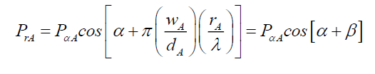 (113)
(113)
This gives and excellent fit (Figure. 4), and suggests that any differences between Airy Pattern ψA (33) and the corresponding probability function PrA (113) are due to experimental error. Comparing (113) with (110) suggests that the photon localizes orthogonally and does not travel along the hypotenuse. Noting the β term in (113) and by (110),

Figure 4: Airy Disc Intensity and Probability.
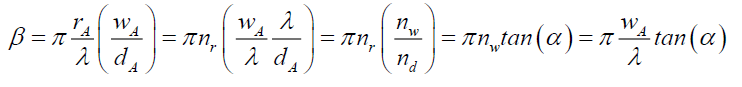 (114)
(114)
Or,
 (115)
(115)
Where nr is the number of wavelengths λ across the Airy Pattern at radius rA, nw the diameter of the pin hole in wavelengths, and nd the distance to the Airy Pattern in wavelengths. However, from (89) the geometry of (116) shows that rh is the horizontal distance in front of the pin hole.
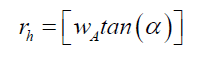 (116)
(116)
 (117)
(117)
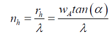
And therefore, the number of wavelengths nh of this distance rh represents a second phase shift forward, introduced by the pin hole of width wA, such that this
 (118)
(118)
And,
 (119)
(119)
That is, photon phase α causes two shifts on the Airy Pattern such that,
• An angular shift θ=α away from the pin hole axis.
• The pin hole causes forward or backward shift of (the non-integer part of) β=nh wavelengths, equivalent to the photon moving forward or backward from the pin hole.
• The photon does not travel along the hypotenuse but localizes orthogonally along the radius rA.
• Localization preserves the total phase shifts α+β.
• The Airy Patternii can thus be explained in terms of photon phase and photon wavelength, and significantly raises the possibility that experiment 11.2 will be vindicated.
Airy Pattern Applications
To test the validity of this, paper photon probability thesis, some experimental tests/applications are suggested.
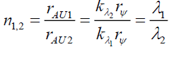
Test 1: The first is refractive index. Since EH is due to the external material of the pin hole, one could propose that the maximum dispersion occurs at rAU1 and rAU2 due to materials 1 and 2, having electric fields EH1 and EH2, and wavelengths λ1 and λ2, respectively, is the refractive index, n1,2.
From (36) and (84),
 (120)
(120)
For the same light photon of frequency ν, and respective velocities v1 (=λ1ν) and v2 (=λ2ν), gives
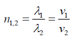 (121)
(121)
This is the correct definition of the refractive index n1,2, thereby confirming the validity of these Airy Pattern calculations. Test 1 passed.
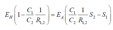
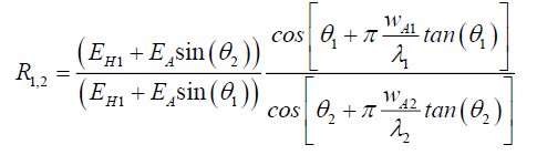
Test 2: The second application is to determine electric field amplitudes. Therefore, considering the ratio R1,2 of the Airy Pattern probabilities, from (97), (107), (114) and (119),
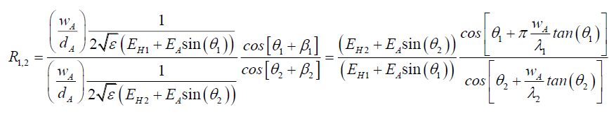 (122)
(122)
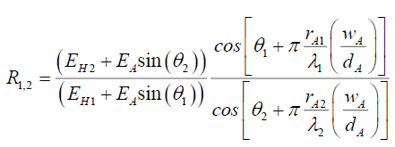 (123)
(123)
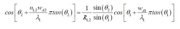
Since the trigonometric function have measurable parameters, these can be replaced as follows,
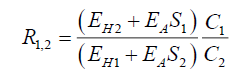 (124)
(124)
Or,
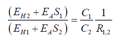 (125)
(125)
for the same medium, but say for the second ring at rA1 and fourth ring at rA2
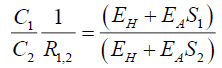 (126)
(126)
Or
 (127)
(127)
Therefore, it is possible to determine the maximum electric field amplitudes from a series of experiments. The key would be to measure the ratio R1,2 sufficiently accurately. Test 2, proposes a new demonstrable experiment.
Test 3: Therefore, the third experiment, given a photon source, is to measure the average space wA between molecules, by replacing the pin hole width wA1 in air with a thin sheet of material 2 whose measurement of spaces between molecules wA2 is of interest, such that its thickness <πnh (93) so that it behaves like a pin hole. From (121) and (122),
 (128)
(128)
And assuming, in air EH1≈0,
 (129)
(129)
And from (116), and (120),
 (130)
(130)
Solving with the known parameters gives average wA2. Test 3 proposes a new demonstrable experiment.
Test 4: Per (107) the phase shift of photons arriving from a pin hole is a function of its orthogonal displacement from the pin hole axis of propagation. Test 4 proposes a new demonstrable experiment.
Test 5: A single phase light beam (e.g. laser) at phase shift α=0° should provide a sharper image than regular diffused light. Test 5 proposes a new demonstrable experiment.
Test 6: Similarly, using this photon probability thesis, it is suggested that it is possible to improve photon detectors by altering the photon’s probability distribution using an external electric field EH required to reduce the photon probability’s upper bound radius rAU to match the radius of the detectors opening. Test 6 proposes a new demonstrable experiment.
Edge Probability Transformations
Given that the Probabilistic Wave Function ψP (50) is not integrable, the integral of the Probabilistic Wave Function ψP (50) does not converge, and therefore the question how does a non-convergent physical process generate the convergent Airy Pattern? Assuming that the photon’s probability function is essentially similar to the Airy Pattern, one can use the Airy Pattern to reconstruct the photon’s probability function in parts.
One can review the coefficient part of the trigonometric function, PαA (97), and PrA (115). These are the projections of the photon probabilities. The former is the pin hole altered photon probabilities at the pin hole, and the latter is the resulting phase shift photon probabilities at the Airy Pattern screen. Therefore, what remains are PEA (95) and PNA (93). (95) is the photon probability in an external electric field, and one is left with PNA (93) which is constant along the photon radius rP, and still a function of the Airy Pattern setup parameters, therefore not quite usable as is.
 (131)
(131)
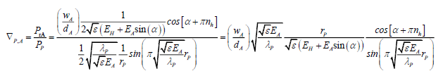
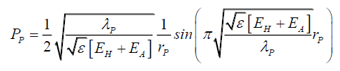
Therefore, using the form of the Airy Pattern function as the basis the solution to the Probabilistic Wave Function ψP (132) is,
 (132)
(132)
 (133)
(133)
 (134)
(134)
 (135)
(135)
 (136)
(136)
 (137)
(137)
 (138)
(138)
And by (110) and (112)
 (139)
(139)
That is, photon probability is a function of the square root of its wavelength λ. Therefore, the true probabilistic transformation ∇P,A caused by the pin hole or for that matter any edge on the photon probability is, (Figure. 5)

Figure 5: Particle Functions versus Radius. Note, some scaling added to display all curves on the same graph.
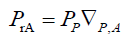 (140)
(140)
Or, from (95), (117) and (145),
 (141)
(141)
Photon Probability Applications
A review of (139) shows that in free space the photon probability is very stable, and therefore an edge transformation ∇PA (140) and (141) is required. Considering (142) one notes that the electric field component could be altered in a manner similar to (95), at least approximately, to introduce the external electric field EH into the photon probability (139). Thus,
 (142)
(142)
Using the vector form of the photon’s electric field EA shows that the maximum effect of the external field occurs when this field is parallel or anti-parallel to the photon’s and therefore, a means to filtering photon by their electric field orientation.
Thus, by (142), when two photons are bound by some process one could propose that the external electric field EH is that of the other photon, and assuming both photons have the same electric field EA,
 (143)
(143)
And therefore, in general with n bound photons,
 (144)
(144)
That there is a phase shift in the set of bound photons and a narrowing of the collective photon probabilities by a factor of √n. This shows that, the edge transformation ∇PA causes the photon probability to phase shift and change magnitude, which is experimentally verifiable. Also, note that the change in the electric permittivity ε will cause a phase shift and a change in the amplitude. Finally, probabilities are affected by velocity and accelerations as the photon wavelength λ undergoes Doppler and gravitational transformations. Gravitational transformations have the additional effects of altering the photon radius rP.
Proposed Experiments
This paper proposes 4 new experiments that photonics researchers can conduct to confirm or disprove the Probabilistic Wave Function ψP (132) and probabilistic control hypothesis presented in this paper. Since, the basic structure of a photon consists of Probabilistic Wave Function ψP (132), the space wave χP (133), and the envelope probability density function φP(134), one can propose tests for the existence of the space wave χP, and the properties of subspace.
Test for altering the probability function
Figure. 6. depicts a possible Airy Pattern experimental set up to prove (142). On the left side is a regular Airy Pattern experiment. On the right side is the corresponding Airy Pattern experiment with the addition that the photons have to pass through an electrical field with field lines in a vertical orientation. By (142) it is opined that vertically oriented photon electrical field would be more influenced than horizontally oriented photon electrical field. There by resulting in vertical deformation with no horizontal deformation. Ultimately, only experiments can confirm or disprove this thesis (142) and provide empirical date to develop probability deformations in the presence of electric and/or magnetic fields. Note, that (153) provides some guidance as the external field strength required in the experiments.

Figure 6: Suggested photon probability deformation in the presence of an electric field.
The next challenge is navigating photons. That is, how to control where to localize. Just as field forces [12,13] require vectoring and modulation, there are two parts to this challenge, (i) vectoring, controlling the direction of localization, and (ii) modulation, controlling the distance to localization. Equation (142) suggests that a spatial gradient of the electric and magnetic fields and the orientation of this gradient could be an approach to vectoring and modulation experiments. This would require a much more sophisticated understanding of subspace. These challenges are left to future research.
Test for space wave particle design that is independent of mass
This relies on the assumption that both mass-based and massless particles consist of this same structure, (132), (133) and (134) with differing coefficients. Would a double slit experiment, with electrons passing through one slit and photons passing through the other slit, both with similar de Broglie wavelengths, produce interference patterns?
Test for space wave χp as the source of self-interference
Can a space wave χP regenerate as two new space waves χPL and χPR? In single photon, double slit experiments, the particle’s path is usually midway between the slits. Shifting this position laterally or sideways, with respect to the slits, should demonstrate a phase shifted interference pattern that is governed by this lateral shift. The resulting interference pattern should be governed by the radial displacements rPL and rPR of the double slits from the photon’s axis of motion. Noting, too, that the wavelengths at the respective left and right are changed per (133).
Since the particle’s axis of propagation is between the double slits, the inference is that the particle does not travel through the barrier between slits because the slits exists. The photon barrier between the double slits should confirm this. Thus, a photon barrier is defined as an obstruction that prevents the formation of the space waves χPL and χPR (not the particle’s χP) in the vicinity of the photon’s envelope probability density function φP (134).
Measuring the Amplitude AP of the Space Wave χP
If the space wave χP has a measurable amplitude AP , then a bidirectional double slit experiment could be used to measure this amplitude. Figure 7. shows such a set-up.

Figure 7: Measuring the space wave amplitude AP.
The reasoning behind this experiment is that the wave interference patterns only occur when the two space waves χPL on the left and χPR on the right, are in contact with each other. Therefore, starting from far, as the distance dS between the left and right screens is decreased, the Airy Pattern should emerge when the left and right space waves χPL and χPR amplitudes coincide. This distance dS at emergence, is the space waves’ amplitude AP.
Conclusion
This paper proposes a new model for a photon’s wave function and how this wave function is modified/transformed in the presence of external objects or edges. The purpose is to provide research directions that will facilitate new types of photon collection and loss reduction technologies. Thus, many new experiments are provided. As it has been shown that probabilities are functions of electric and magnetic fields, a mechanism for deforming probabilities is proposed. Therefore, probabilities can be controlled.
1http://www.feynmanlectures.caltech.edu/III_16.html
2 http://www.colorado.edu/physics/TZD/PageProofs1/TAYL07-203-247.I.pdf
3 http://hyperphysics.phy-astr.gsu.edu/hbase/oscda.html
4Even though the exponential term +1/u has a positive sign compared to the negative in-γ, the u function is an inverse.
5Regression fitting the data (1/u against exp+1/u) gives R2 of 99.944%, 99.562%, 98.131%, 95.846% and 92.959% at screen distances, ds of 0.10 m, 0.25 m, 0.50 m, 0.75 m and 1.00 m, respectively. Compared to an exact theoretical model producing an R2 of 99.9999%. That is the damped oscillation model fails as dA increases. This implies that a different model is at work.
References
- Nemiroff R. Bounds on Spectral Dispersion from Fer-mi-detected Gamma Ray Bursts. Phys Rev Lett. 2012;108:231103.
- Wong CW. A review of quantum mechanics, review notes prepared for students of an undergraduate course in quantum mechanics. Department of physics and astronomy, University of California, Los Angeles, CA2006; 2016.
- Roychoudhuri C. Causal physics: Photons by non-interactions of waves, CRC Press, Boca Raton; 2014.
- Solomon BT, Beckwith AW. Probability, randomness andsubspace, with experiments. J Space Explor. 2016;6(1).
- Bohm D. A suggested interpretation of the quantum theory in terms of hidden variables, II. Phys Rev. 1952;85(2):180-93.
- Fluid mechanics suggests alternative to quantum orthodoxy [internet]. MIT News [cited on 2014, Sep 12]. Retrieved from: [http://news.mit.edu/2014/fluid-systems-quantum-mechanics-0912]
- Efstathiou G, Pryke C, Steinhardt P, et al. Spotlight live: Looking back in time-oldest light in existence offers insight into the universe. The Kavli Foundation;2015.
- Solomon BT. New evidence, conditions, instruments and experiments for gravitational theories. J Mod Phys. 2013;4:183-96.
- Solomon BT. Non-gaussian photon probability distributions, in the proceedings of the space, propulsion andenergy sciences international forum (SPESIF-10). Glen AR, editors. AIP Conference Proceedings 1208; Melville, New York; 2010.
- Solomon BT. Empirical evidence suggest a need for a different gravitational theory, American Physical Society (APS) April Conference, Denver; 2013.
- Solomon BT. An introduction to gravity modification: A guide to using Laithwaite's and Podkletnov's experiments and the physics of forces for empirical results. 2nd edition. Universal Publishers, Boca Raton: 2012.
- Solomon BT. Gravitational acceleration without mass and non-inertia fields. Phys Essays. 2011;24: 327.
- Solomon BT. An approach to gravity modification as a propulsion technology, in the proceedings of the space, propulsion and energy sciences international forum (SPESIF-09). Glen AR, editors. AIP Conference Proceedings 1103; Melville, New York; 2009.
- Hooft G. A locally finite model for gravity. Found Phys. 2008;38:733-57.
- Solomon BT. Super physics for super technologies: Replacing Bohr, Heisenberg, Schrödinger and Einstein, Propulsion Physics Inc, Denver March; 2015.