Original Article
, Volume: 5( 3)The Mounds of Cydonia: Elegant Geology, or Tetrahedral Geometry and Reactions of Pythagoras and Dirac?
- *Correspondence:
- Crater HW , The University of Tennessee Space Institute, Tullahoma, TN 37388-9700, USA, Tel: 931-393-7469; E-mail: hcrater@utsi.edu
Received: October 04, 2016; Accepted: November 10, 2016; Published: November 30, 2016
Citation: Crater HW, McDaniel SV, Sirisena A. The Mounds of Cydonia: Elegant Geology, or Tetrahedral Geometry and Reactions of Pythagoras and Dirac? J Space Explor. 2016;5(3):105.
Abstract
Based on high resolution images from the ESA Mars express and NASA orbiter HiRise cameras, this paper gives new in-depth analysis of the remarkable geometric distribution of certain "mounds" or hill-like features in the Cydonia region of Mars. It validates the earlier measurements obtained using the lower resolution NASA Viking images, which hinted strongly at artificial surface interventions and adds new information regarding the geometry. We describe how those surface features, if artificial, provide an elegant and concise way for an intelligent species to transmit to another intelligence evidence that it understands the basics of tetrahedral geometry, prime numbers, and the quantum mechanics of the electrons spin, thereby giving additional evidence for the possibility of intelligent intervention. We also explore plausible geological explanations for the individual mounds and survey the possible natural mechanisms which may have been involved in their unusual and mathematically precise positioning.
Keywords
Mounds; Geometry; Electron
Introduction
The use of the prime number series as a way to signal to ET is by now a fairly well-known idea. In the 1997 l m contact, an adaptation of the novel [1] by Carl Sagan, radio telescope researchers discovered a signal containing a series of prime numbers. This led them to conclude it was a probable communication from ET. Toward the end of the book upon which the movie was based, the main character Ellie searches for patterns in π and finds a very long string of 1s and 0s far out in the base-11 expansion of π that when arranged in a square of a specific size yields a clear drawing of a circle and its diameter. One could say that because of the role that π plays for the circle that she has been given a scheme by which the number is rendered self-referent. This could be regarded as a second indication of an ET message. Long before this the idea of somehow depicting the Pythagorean Theorem as a message that could be seen from space was fielded at least as far back as 1900.
The idea was to draw the appropriate geometric figure on the terrestrial landscape large enough so that it might be detected by aliens on the Moon or Mars. A plan for doing so in the Siberian forest, reportedly attributed to Gauss, may date back to 1820 [2], Combining all three ideas, a geometric figure that would clearly reference a series of prime numbers, represent a unique geometric figure such as the Pythagorean Theorem or the geometry of one of the five regular solids such as the Tetrahedron, and in addition have a self-referent property, would certainly qualify as a potentially meaningful communication intended for ET.
In a previous set of papers [3-5] we displayed in some detail our geometric study of the placement of five mounds or hill-like features located in the area known as Cydonia, on Mars. Attention was first drawn to these objects in the 1976 Viking spacecraft photos because they exhibited a noticeably higher albedo than surrounding landforms as well as lying in a relatively open space with no other similar objects nearby. Below are the mounds labeled from Viking image 35A72, (Viking 35A72 (1976) with their positions enhanced for ease of location. Figure 1 and 2 are close ups of this same image (Viking 35A72 (1976)) with added outlines of triangles indicated. Included are several other mounds which later came under consideration.

Figure 1: 12 Cydonia Mounds notated; Viking 35A72 (1976).

Figure 2: Comparison of the mound geometry and the angles of the pentad related to the tetrahedron and to the classic square root 2 rectangles. (Viking 35A72 (1976))
Although the resolution of these early images is low (47 pixels/meter), aside from their brightness, the apparent isosceles triangle EAD also drew attention to the pattern. Using very careful methodology, the indicated geometry appeared to form a figure having just exactly the criteria mentioned above, self-reference, an unmistakable reference to the prime number series 1,2,3,5,7, and an equally unmistakable reference to the geometry of the Tetrahedron.
Although of course such a coincidence might be written off as a freak of unlikely geology, even a hint of such a figure should be enough to arouse considerable scientific curiosity. We feel it would be a mistake to ignore the possibility of artificial intervention without first engaging in a careful analysis. The data must be checked and checked again, the precision of the mound placements determined, the possibility of arbitrary choice of randomly placed features considered, and geological explanations explored. When necessary, methods of procedure for doing this rigorously must be developed. And a serious impediment was the low resolution of the Viking images.
Now, however, we have the benefit of new images. The first is the European Space Agencies, ESA Mars Express satellite image H3253_0000_ND3 released in 2006 with a resolution of 13.7 meters/pixel taken recently by the ESA satellite Mars Express (13.7 meters/pixel) [6] and more recently NASAs HiRISE satellite image D21_035487_2215_XN_41N009W released in 2014 with a resolution of 5 meters/ pixels [7]. These have given us the opportunity to test our original analysis and its degree of precision. The present paper gives our results to date. We begin with a general overview of the significant features, to be followed in the next section with greater detail as to methods employed and results.
Within carefully measured tolerances (see below) the group of five mounds we term the pentad outlines (1) an isosceles triangle whose internal angles match the cross-section of a tetrahedron, (2) right triangles whose internal angles match precisely those produced by taking any altitudes of that same isosceles, (3) one of the angles produced twice within the isosceles by its altitudes is an angle t=19:5 degrees, which is sometimes called the tetrahedral latitude because when a tetrahedron is embedded in a sphere, its base marks that latitude on the sphere, and (4) the five mound configuration can be seen to be clearly related to a portion of a classic geometric figure called a square root of 2 rectangle, which has not only multiple repetitions of these tetrahedral angles but a history in aesthetic proportions as well, and moreover is the only rectangle which, when divided along its center width, produces a replicate of itself and is thereby endlessly self-referent.1 All these characteristics are described in ne detail in reference [8]. Finally, analysis of the relative areas of the triangles contained within the pentad (and the hexad when mound P is added) shows that they represent the prime numbers 1,2,3,5 and 7. Below we place a composite image of the pentad of mounds GEDBA, rotated and cropped from Figure 1 alongside the idealized version within the square root of two rectangles. The letters I, H, F, do not represent mounds but rather the points of symmetry in the implied rectangle. Points I, H, A, E, F mark an inverted mirror image of the pentad. Points C and X are key locations in the corresponding tetrahedron (Figure 2). 1 The A4 paper size used in some parts of the world is actually a selfreplication  grid.
grid.
As the name implies, a square root of two rectangles has a ratio of the long side to the short side equal to . Thus, in the above figure if DB has the length of 1 then BA would have the length of . The length of GE is also equal to . In addition to the above Viking representation of the pentad from image 35A72 in 1997, depicted below are the corresponding images from the Mars Express. Figure 3 and 4.

Figure 3: Pentad in ESA Mars Express image H3253_0000_ND3 (2006) and Hi Rise satellites.
[Available from: http://www.esa.int/spaceinimages/Images/2006/09/Cydonia_region_colour_image2]

Figure 4: Pentad, MRO HiRISE CTX D21_035487_2215_XN_41N009W (2014).
[Available from: http://viewer.mars.asu.edu/planetview/inst/ctx/D21_035487_2215_XN_41N009W#P=D21_035487_2215_XN_41N009W& T=2
The corresponding images display the mounds as they are with no enhancements. Because of the difference in sun angles, the higher resistivity of some of the mounds is not as pronounced as it is in Viking 35A72.
Methodology and Analysis
In our most recent paper we focused only on the pentad of mounds. Here we will include a sixth mound, designated as mound P, so our analysis will be on what we call the hexad. We will also give an expanded account of the mound geometry, particularly in its relation to the tetrahedron, and the quantum mechanics of the electron spin. The image we used from Viking is an orthorectied version. By that it is meant that the at image is portrayed as if shot from directly overhead, even though the actual satellite image may not be from directly overhead. The image from the Mars Express satellite used in the recent paper [5] was taken almost directly overhead and there was no need for orthorectication. In this paper, we report the results of the re measurement of the angles for the triangles in the pentad and the resultant coordinated t (to be defined below), from a map projected image that was not from directly overhead. For areas, as small as the ones that we are considering there is no significant difference between a map projected image and an orthorectied image.
To avoid arbitrary selection of the points within the mounds where the vertices of the triangles meet, we used a coordinated fit, which is implemented by a computer program. To get a visual picture of what the program does, imagine that each mound is represented by a rectangle. Within each mound one places a point (initially at the center). A coordinated fit requires that the same vertex within any given mound is used for all the triangles having one vertex sharing that mound, not shifted about arbitrarily within each mound to accommodate each triangle separately. In that sense of the word the triangles are coordinated. That is, their vertices are not placed at arbitrary separate points within each mound with one point for each triangle that has a vertex within the mound. Another way of stating this is that the five-sided figure that represents the pen-tad is closed. Now what the computer program does is to vary those common vertices away from the centers but within the confines of each mound so as to obtain a best possible fit to the ideal angles as to be given below. A precise coordinated fit to the ideal angles (within 0.2°) with common vertices lying within the mounds was obtained with 35A72 in 1997, and here we report a similar coordinated fit 0 the ideal angles achieved with the Mars Express and HiRise images. In the Appendix we present the initial set of angles obtained from the estimated x and y coordinates of the centers of each mound for each of the three sets of images as well as the ideal angles.
It is not a given that such a t can be obtained. In fact, in [9,3] we found that it is extremely unlikely given five or more randomly placed mounds of size similar to the Cydonia mounds, that such a t to the ideal geometry can be obtained. One might ask why did we choose this particular geometry. As explained in the previous papers if one plots the number of right and isosceles triangle obtained from a coordinated fit versus an angle t defined such that the angles in radians for the right triangles are π/4-t/2, π/2, π/4 + t/2 and for the isosceles, the ideal angles in radians are π/4+ t/2, π/2-t, π/4+t/2, then by far the most right and isosceles triangles appear among the Cydonia mounds when t=arcsin (1/3) ( 19:5°): In other words the Cydonia mounds chose this geometry far above any other. So, given this choice of the t angle we focus on the pentad.
Prime numbers and the pentad
Consistent with the idea of a "message", the mound geometry is profoundly pedagogical with respect to the connection between the concepts of number and size, both in terms of length and area. One’s first experience with numbers is basic counting, not magnitude of length and area. It is almost as if the (hypothetical) builders of the pentad were taking special pains to display the basic connection between concepts of number and magnitude of length and area. Consider the following images of the pentad of mounds taken from our recent JSE paper [5]. The mounds (GEDBA) are highlighted for clarity. The right triangles DBA, BAE, GEA, and DAG are all similar (having the same angles). This is shown explicitly in the diagrams below. Having exactly the same side and angle measurements, clearly the triangles GEA and BAE are congruent right triangles Figure 5.

Figure 5: Congruent triangles of the pentad. Viking 35A72 (1976).
In the next figure the right triangles DAG and DBA are similar not only to each other but they are also similar to the above congruent right triangles Figure 6 and Figure 7.

Figure 6: 2 Further similar right triangles, Viking 35A72 (1976).

Figure 7: Isosceles triangle of the pentad; Viking 35A72 (1976).
The next figure shows the related isosceles triangle ADE. This isosceles triangle is the double of the right triangles DBA.
All the subsequent features that we will describe follow logically and mathematically from the ideal geometry which their placements portray. It is our opinion that those features, if the placement of the pentad of mounds was intentional and not natural, display a characteristic of the intelligence that placed them that may best be described by the words pedagogically clever. Consider first of all the relative areas of these right triangles. We shall show that the pentad of mounds displays the concept of area in a self-referent way and also with a correspondence to the first 4 prime numbers. By self-referent in this regard we mean that the area of the pentad, a five-sided figure denied by five mounds, has simultaneously an area of five units. To see this and the claim about prime numbers let us take the area of the smallest of the similar right triangles to be one unit as shown in the Figure 8 to the left below. Since the base of the intermediate sized congruent right triangles is twice that of the smaller one and its height is the same, its area is of course twice the area. But why is the area of the largest of the four similar right triangles three times that of the smallest one?

Figure 8: Relative areas of similar right triangles; Viking 35A72 (1976).
That is explained by reference to Figure 2 and the rectangle. Since the hypotenuse of the smaller right triangle is, from the Pythagorean theorem,  times its base, this implies that the base of the large right triangle GAD is times the base of the smaller triangle. The height of the large triangle is the length of the line GA which is the diagonal of the square root of two rectangle GHAE (Figure 2). Since the base of that rectangle is times its height, the diagonal of that rectangle will be p3 times its height. Since its height of that rectangle is the same as the smaller triangle ABD, the height GA of the larger right triangle will be times that of the small right triangle. Thus, since both the height and the base of the larger triangle are times that of the smaller triangle the area of the larger right triangle will be 3 times the area of the smaller triangle Figure 8.
The sizes of these three similar right triangles thus correspond to the first three prime numbers. It is thus all the more remarkable as seen in the figure below Figure 9. that the next prime number 5 appears as the area of the entire five-sided pentad. The source of this geometrical wonder (in the sense of either extraterrestrial interventions or geological formations) displays this prime number in a self-referent way, roughly analogous to the way is described in a self-referent way in the introduction. As seen from Figure 8. we also have with this scale that the obtuse triangles EDB and GED each have unit area. And, since the area of the tetrad of mounds GADE is 4 we have a self-referent 4-sided figure nested inside a self-referent 5 sided figure. To top this off, since the triad of mounds GAD has an area of 3 we have a self-referent 3-sided figure nested within a self-referent 4 sided figure nested with in a self-referent 5 sided figure.

Figure 9: Relative area of the pentad; Viking 35A72 (1976).
Before going on to the hexad and the next prime number let us consider lengths. The geometry parallels the basic 1,2,3 sequence of areas with the same sequence of lengths of pertinent sides of the triangles relative to one another. Let us again take the shortest side (BD) of the smallest triangle (ABD) to be 1. Then, with our ideal geometry, the middle side (EA) of the middle sized triangle (GEA) is 2, and the longest side (GD) of the largest triangle (GAD) is 3. As the figure below emphasizes, in sequence of size of the triangles ABD, GEA and GAD from the smallest to the largest, the three basic aspects of the sides of a right triangle: opposite and adjacent to the smaller acute angle, and hypotenuse, are ordered 1,2,3 sequentially with their side lengths (opposite of ABD, adjacent of GEA, and hypotenuse of GAD) Figure 10.

Figure 10: Increasing lengths of 1,2,3; Viking 35A72 (1976).
This 1,2,3 sequence is repeated a third time in the ratios of the sides of each similar right triangle of  . The geometry is indeed clever and persistently pedagogical.
The hexad and the prime number 7
Let us now consider the consequences of the addition of mound P to produce the hexad of mounds below Figure 11 and 12. Even the two congruent obtuse triangles GEB and BAG participate in this 1,2,3 pattern. Using the BD=1 scale in Figure 10. and the Pythagorean theorem, the lengths of the sides GE, EB, and BG of the GEB and BA, AG, and GB triangle work p out to be respectively  . For the experts, note that the GEB and BAG triangles corresponds in quantum mechanics to the addition of angular momentum 1 plus angular momentum 2 to give angular momentum of 3 since the magnitude of angular momentum S is
  .
.

Figure 11: The Hexad of mounds from Viking 35A72 (1976).

Figure 12: Hexad displaying similar right triangles, Viking 35A72 (1976).
[Available from: (http://www.esa.int/spaceinimages/Images/2006/09/Cydonia_region_colour_image2)
We have found in previous work that the placement of this mound leads to an additional right triangle that is strictly congruent with the triangles DAG and EAB. The Viking Figure 12 below displays this explicitly. We were able to obtain a coordinated fit for the hexad of six mounds with the ideal geometry and now five similar right triangles. They are the triangles labelled GAD/ABD/EAB/AEG/PGE. The latter three are congruent. There is also an isosceles triangle EDA and seven sets of parallel lines PG?EA, PE?GA, PG?DB, GE?AB, GA?EB, DB?EA, and GB?ED. Finally, GABE and PGAE form two parallelograms. Here we see these properties with the lines below. Since in the units portrayed above, the pentad has an area of 5, the hexad has an area of 7. The reason is that the triangle PGE that extends off the pentad to make the hexed is congruent to the triangle GEA which in the units portrayed above has an area of 2. Thus, the area of the hexad PGABDE in these units is 7, the fifth prime number. One of the criteria for artificial origin listed in [8] was whether the resulting geometry is unproductive, or rich. This propensity toward indicating the prime numbers is one thing that makes the pentad and the related  rectangle rich.
As a further indication of this propensity, consider first that all the similar right triangles of the pentad have their sides taking on the ratios of  . If we take the smallest of them to be scaled so that
  then of course it’s other two sides are
  . Recall that the two congruent right triangles would then have their sides in the ratios of
 . Now consider the smallest of the similar right triangles. The square of its small side is obviously 1. The square of the middle side is 2. Add the square of the short side to the square of the middle side and of course the Pythagorean theorem gives us 1+2=3.
The coordinated fits obtained with the above cropped portion of the 1997 Viking image 35A72 was repeated with the higher resolution Mars Express image.
Now jump to the congruent right triangles. Then starting with the prime number 3 from the sum 1+2, all of the prime numbers from 5 through 89 can be obtained by adding the three even numbers 2 or 4 or 6 corresponding to the squares of the sides of the middle sized right triangle (which of course satisfy 2+4=6). So, 3+2=5, 5+2=7, 7+4=11, 11+2=13, 13+4=17, 17+2=19, 19+4=23, 23+6=29, 83+6=89. This prime number generating feature of the  right triangle runs out of steam here since the next prime number is 97=89+8.
Of course this string of successes is simply due to the fact that all of those intervening prime numbers are related to their nearest neighbor by the addition of either 2 or 4 or 6. What is rather curious and interesting is the connection between 2,4,6, and the Pythagorean theorem applied to our congruent tetrahedral right triangles. This fact lies, of course, in the context of the prime numbers 1,2,3,5,7 that we obtain from the areas of the tetrahedral right triangles of the pentad (and hexad) Figure 13 and 14.

Figure 13: Mars Express hexad image. ESA Mars Express H3253_0000_ND3 (2006). [Available from: http://viewer.mars.asu.edu/planetview/inst/ctx/D21_035487_2215_XN_41N009W#P=D21_035487_2215_XN_41N009W&T=2]

Figure 14: MRO HiRISE hexad image. MRO HiRISE CTX D21_035487_2215_XN_41N009W (2014).
The tetrahedron and tetrahedral triangles of the hexad
The remarkable geometrical and prime number properties of the pentad and hexad follow from the corresponding geometrical properties of the square root of two rectangles. Those geometrical and prime number properties are a logical outcome of the relative placement of the mounds and are not independent of those placements. This would hold true for any subsequent theoretical discovery related to those placements. For example, the connection between the pentad and electron spin discussed in the next section is such a theoretical discovery and a consequence of an already discovered property of the relative placements of the mounds. By contrast, the placement of mound P has both new and supportive consequences for the properties of the pentad of mounds. It is new in that it involves a mound separate from the five mounds of the pentad. It is supportive in that it not only leads to a coordinated fit with a fifth right triangle similar to the four right triangles of the pentad, but it is also placed in such a position as to accentuate the square root of two rectangles inferred from the pentad. The figures below demonstrate this explicitly, in the Viking, the Mars express image Figure 15-17.

Figure 15: The Mars Express image of the extended rectangular grid. ESA Mars Express H3253_0000_ND3 (2006). [Available from: tp://viewer.mars.asu.edu/planetview/inst/ctx/D21_035487_2215_XN_41N009W#P=D21_035487_2215_XN_41N009W&T=2].

Figure 16: The HiRISE image of the extended 2 rectangular grid. MRO HiRISECTXD21_035487_2215_XN_41N009W (2014).

Figure 17: The Tetrahedron and its isosceles cross section.
(http://www.esa.int/spaceinimages/Images/2006/09/Cydonia_region_colour_image2)
They show not only the rectangular grid in which the pentad is embedded but an extended square root of two rectangular grid. The proportions of the triangles involved are connected directly to the value of the angle t which defines the angles that appear in the similar right triangles π/ 4- t/ 2, π/ 2,) and the isosceles triangle π/ 4+ t/ 2, π/ 4 + t/ 2. As mentioned in the introduction, the isosceles triangle has internal angles which match precisely those of the cross-section of a tetrahedron. This is seen in the figure below in which the shaded area with vertices ADE corresponds to that triangle Figure 17.
Now we discuss two further mounds, whose placements bear further intriguing connections to the tetrahedral triangles and the tetrahedron. The first mound we discuss is mound M (Figure 1 and 18). We have obtained coordinated fits that involve this mound and all six mounds of the hexad. That coordinated fit reveals an isosceles triangle PMA that is similar to the triangle ADE and of course the cross-section of the tetrahedron. As the three figures below show from the Viking, the Mars Express in Figure 18-20.

Figure 18: Mound M with Isosceles PMA Similar to ADE and Mound O with Equilateral OPG; Viking 35A72 (1976).

Figure 19: Mars Express image of Mound M with Isosceles PMA similar to ADE and Mound O with Equilateral OPG ESA Mars Express H3253_0000_ND3 (2006).

Figure 20: HiRise image of Mound M with Isosceles PMA similar to ADE and Mound O with Equilateral OPG. MRO HiRISE.CTXD21_035487_2215_XN_41N009W (2014).
(http://www.esa.int/spaceinimages/Images/2006/09/Cydonia_region_colour_image2), and the HiRise satellites http://viewer.mars.asu.edu/planetview/inst/ctx/D21_035487_2215_XN_41N009W#P=D21_035487_2215_XN_41N009W& T=2 coordi-nated fits.
not only reveals that the triangles are similar, but also that their respective bases’ display the opening angle t; from the shared common vertex A, which defines the geometry of the tetrahedron and the tetrahedral angles and triangles. The area of that triangle is 9/2 the area of the triangle ADE [10]. This follows from the fact that a) the two triangles are similar and b) the base of the triangle PMA q, in units in which BD=1, is  . Since the two triangles are similar, the height of the larger triangle would also be
  times that of the smaller triangle. The square of this common factor is 9/2.
With the ortho rectified Viking data we were able to obtain a coordinated …t that not only displays the above additional isosceles PMA but also, including mound O, shows that the triangle OPG is equilateral. This triangle is quite significant in terms of its connection with the tetrahedron in Figure 17.
Since the base PEG for the equilateral has the same length as the base AE for the isosceles cross-section ADE, this means that the ratio between the area of the equilateral OPG and the isosceles ADE is precisely the same as the ratio between the area of each of the four sides of the same tetrahedron which includes the triangle ADE as its cross-section. Unfortunately, even though we were able to obtain with the Mars Express and Hirise images a coordinated fit for OPG with angles very close to the equal angles of 60° we were off by about a half a degree. This discrepancy between the different images may be due to the satellite angle: neither the Mars Express nor the HiRise images are strictly speaking orthorectified. However as mentioned earlier the Mars Express image was taken almost directly from overhead which at least approximately fits the definition of what we mean by an orthorectified image. The HiRise image was map projected, not the same as an orthorectified image but close.
The mound geometry and the electron spin
As reported in earlier papers [3,5] the right triangles pictured above are of importance in the fundamental physics of the spin of the electron (and the quark). It was Goudsmit and Uhlenbeck who in 1925 proposed that the electron has an intrinsic angular momentum apart from its orbital angular momentum that it may have in rotating about the nucleus of an atom. In 1929 Dirac found the relativistic wave equation for the electron bearing his name, confirming the fundamental nature of electron spin. His theory showed that the electron spin could be described by a single quantum number s whose value could only be s=1=2. The other important aspect of Dirac’s equation is that it predicted the existence of the electron’s antiparticle, the positron, a particle with the opposite charge of the electron but with the same intrinsic spin.
Let us begin with a naïve picture of the spinning electron as that of a top [11]. In the playful picture below we have two pictures of an electron which corresponds to our experiences of a spinning and processing top on a table in the constant gravitational field of the Earth. This picture of the electron is naïve in several respects. First of all the electron as far as we know has no size. That is, it is a point particle. So how can an object with no size have a spin? The fundamental equation of physics that describes the electron and it’s spin is the Dirac equation. In the case in which there are no electric or magnetic fields to act on the electron and it is at rest, the Dirac equation tells us that its energy is simply E=mc2. This is the same energy a particle of mass m would have even if it had no spin. There is no room in this famous equation to account for the rotational energy that the electron would have if it had extension like a top [4]. On the other hand if a constant magnetic field.
4For an ordinary top with spin S and moment of inertia I, the rotational kinetic energy added to E=mc2 would equal to S2=2I: is turned on then the electron picks up an energy over and above mc2 even if the electron is at rest. The Dirac equation tells us that this energy arises from the orientation energy of the electron with the magnetic field by way of a tiny magnet intrinsic to the electron and directly proportional to its spin. So, the electron behaves like a tiny permanent magnet whose orientation defines an axis and whose strength is proportional to its rate of spin about that same axis. In our figure the electron is shown as having 2 ways of spinning about that axis, one clockwise one counterclockwise. Instead of the gravitational field pointing straight up for a real top, we have the electron spinning and processing in a constant magnetic field pointing straight up. The peculiar thing about the electron is that the angle that it’s spin axis makes with respect to that constant magnetic field can take on only two values. To get a hand on what we mean by orientation use your hand. For the picture on the left you grab that top with your right hand in such a way that your four fingers curled around the top in the direction of the arrow. Then the orientation of the spin, of the magnet, of the electron points in the direction of your thumb. For the electron to the right if we do the same thing with your hand, then your thumb would point down at an angle relative to the vertical, that is to say relative to the direction of the constant magnetic field. The thing about the electron, unlike a toy top, is that the angle of the spin axis relative to the magnetic field can take on only two values, corresponding to the two directions of your thumb. Furthermore, the magnitude of the spin about the axis is fixed and permanent, just like the permanent magnetism of the electron Figure 21.

Figure 21: Electron spin, naive picture.
Let us translate this into a picture that will allow us to see the relevance of the right triangles that appears five times in the hexad. Planck’s constant h plays an important role here. Quantum mechanics stipulates that the magnitude of the electron’s spin is given by  . Its magnitude and direction are represented by the red arrows in the figure below Figure 22. The two red arrows correspond to the two possible spin orientations of the electron. The arrow that points upward and to the right represents the axis of the electron and in the presence of the magnetic field this arrow processes about the z-axis [12]. Its projection about the z-axis is fixed, having only the possible value of
  (the factor of 1/2 here authors the description of the electron as a spin-one-half particle). In the picture above this corresponds to the purple top. The arrow that points downward to the right represents the axis of the electron and in the presence of the magnetic field in the z-direction this arrow processes about the z-axis. Its projection about the z-axis is fixed, having only the possible value of -
 . In the picture above this corresponds to the blue top.
Now even though this picture is taken as representing the dynamical picture of an electron processing and spinning in and out of the page in a magnetic field let us view just this cross-section as is pictured. Now consider the two triangles pictured with each of the red arrows corresponding to a hypotenuse, the projection of the spin along the z-axis representing the small side of the triangle and the other projection representing the intermediate side of the tri-angle. (From the Pythagorean theorem, the magnitude of this other projection, p that is, the dotted line is given by  ). It is impossible that the electron p can have a magnitude of the spin any other value that value of
  . It is impossible that its projection along the z-axis be other than ± (remember the z-axis represents a direction of a constant magnetic field applied in our lab-oratory about which our electron is spinning and processing). It is impossible to increase the spin rate or decrease the spin rate Figure 23. That is a permanent feature of the electron. The lengths of the sides of the two triangles represented are
  ). The proportions
  correspond precisely to the proportions of the lengths of the sides of the five similar right triangles of the hexad. Using the ideal angles of the right triangles of the hexad, the two possible angles of orientation are + π/4- t=2) 35:3 degrees and - π/4-t/2 35:3 degrees, above and below the horizontal. Let us make this correspondence between the spin of the electron and the mound configuration more vivid by using the pictures of the mounds themselves.

Figure 22: Intrinsic spin angular momentum for electron.

Figure 23: Mound geometry and electron spin; Viking 35A72 (1976).
Here we see clearly the precise correspondence between the mound configuration and the electron spin. The short side DB in this figure corresponds to the z-axis projection in the previous figure. The circle here in this figure corresponds to the processing red arrow in the previous picture and the line AB in this figure corresponds to the dotted line in the previous picture. The lengths BD, BA, and AD have the respective ratios of (). The blending of mound geometry and quantum mechanics on the surface of Mars does not end here.
Consider the two equal legs DE and DA of the isosceles triangle pictured in Figure 7. They each process about what would be the magnetic field direction DB if we were speaking of a processing electron. In quantum mechanics when two spin-one one half particles such as electrons or quarks combine their spins, they can add to an overall spin-zero (S=0) or spin-one (S=1). When they combine to spin-zero, there is a net zero magnetism that is produced. However, when the spins combine to give a total spin one (S=1), that gives the maximum composite magnetism. In that state the relative orientation of the two spins is the same as that between DE and DA, corresponding to an angle of π/2 t=70:5 degrees [13]. In Figure 24 opening angle is represented by the angle between the two cones. The designation MS=0 indicates that the net spin component about the z-axis is zero. The upper blue arrow and the lower process in opposite directions.

Figure 24: Composite spin-1 state for 2 spin-one half particles.
In the figure below this is shown in the context of the actual Cydonia mounds (that figure is rotated π/2 relative to the figure above). The two individual electrons correspond to the red arrows, giving rise to a total spin of magnitude h corresponding to spin 1(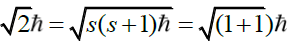 represented by both the length and the direction of the yellow arrow. Note that the yellow arrow has a zero projection along the z-axis in the figure (along DB) corresponding to MS=0.
The Pauli exclusion principle would forbid such a spin-one state between two electrons if they are in the same orbital. For example, 2 electrons in the ground state of helium could only couple to give spin zero not spin 1. But this figure does not represent spin zero for which the two blue arrows would be antiparallel rather than at an angle of 70.5 (= π/2-t). So if this were to represent some bound state involving two electrons this could only be possible if say one of the electrons is in a ground state and the other is in another orbital, say the first excited state. The alternative is that one of the spin one half particles is not an electron but a positron, or an anti-electron. In that case, we would have represented here a bound state of an electron and a positron corresponding to what is called triplet positronium or ortho positronium. Symbolically it corresponds to S1. The designation triplet corresponds to the fact that the diagrams here correspond to only one of three different states in which the positronium atom could be found in. In the other two states, not represented by the Cydonia mounds, the two blue arrows would be circling around in just one of the cones, either the upper or the lower with the angle between them being fixed again at 70.5° Figure 25.

Figure 25: Composite spin state displayed by mounds; Viking 35A72 (1976).
There is a fourth composite spin state for the positronium system. In that state the total spin is zero (S=0). The diagram [13] representing it is given in the figure below in Figure 26.

Figure 26: Composite spin state for total spin zero.
As the arrows in the figure indicates the two electron spins are in opposite directions so that the spins cancel to zero. One precesses on the top cone and the other on the bottom cone. Strictly speaking if the mound geometry here were to represent a spin-zero composite, then line DE would point in the opposite direction to line DA as in the figure above. However, there is an indirect way in which the spin-zero composite is represented by the side EA. First note that the length of each spin vector for each electron is /2. Thus, magnitude of the total length of the double arrow is . The angle that each of these double arrows make with the vertical axis is π /4 + t/2 which is one half the angle between the two cones of π/2-t. The projection that this total length would make on the vertical is the length times the cosine of that angle.
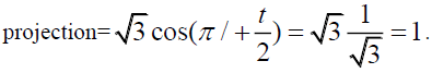
On the scale, we have represented in Figure 10 with DB= 1 instead or 1=2 the spin lengths (DE and DA) are represented by p3 instead of their actual lengths of /2. Because of this doubling of scale in his figure, the projection would be of magnitude 2 instead of 1. That magnitude of 2 is represented by the length EA in that same figure. Of course, there are no lines actually on the planet much less arrow tips pointing in opposite directions but that 2 does represent the length of the doubled arrowed line in Figure 26. One should not confuse the magnitude of that projection with the actual spin which is zero. So, in this sense the pentad of mounds represents both composite spin states of the positronium system. The two angled lines DE and DA correspond to the triplet state 3S1 whereas the line EA represents the singlet state S0. The letter S refers to the fact that the electron and positron have no orbital angular momentum about one another (in this S-state the probability cloud that quantum mechanics predicts is a sphere not a circular orbit). The two subscripts 1 and 0 correspond to the total angular momentum (spin and orbital) of 1 and 0 respectively. The left placed superscript describes the number of different possible ways that the electron and positron could combine to give the respective total spins of 1 and 0.
The Geology of the Mounds
Possible origin of the mounds
The above considerations might suggest an artificial intervention in the mound placement. Despite the consistently repeating coordinated fit, the mounds themselves do not have an obviously artificial appearance, although they may have been subject to long-term erosion over a great length of time. So, what might geology tell us about a possible accidental or coincidental distribution of the mounds to form just this geometrical pattern?
SPSR member and geologist Peter Ness has kindly provided us with his evaluation of the possible geological origins of the mounds. Based on detailed images of the mounds from the HiRise satellite he states most of them are likely mud mounds and refers to them as such in the descriptions below. (See appendix for definitions of various technical geological terms).
Location of the mounds: The mud mounds are located near the base of the 24-Feb-2014 regional Mars Orbiter context image (Figure 27). This image, which is centered on latitude 41.49 N, longitude 350.15W, is the regional image containing the same geology as the HIRISE images discussed in this paper:

Figure 27: Mars Orbiter Context Image showing the area containing the mounds (RHS), MRO HiRISE CTX D21_035487_2215_XN_41N009W (2014). North is to the top of the image.
http://viewer.mars.asu.edu/planetview/inst/ctx/D21_035487_2215_ _41N009W#P=D21_035487_2215_XN_41N009W&T=2 Cydonia mud mounds A, B, D are from HIRISE image http://www.uahirise.org/ESP_025505_2210, taken on 04-Jan-2012, centered on 40.520 N, 350.359 E with a resolution of 0.5 m/pixel. Mound P is located near the top and Mound B toward the base of HIRISE image.
http://www. uahirise.org/PSP_005924_2210 taken on 01-Nov-2007, centered on 40.526 N, 350.095 E and has a resolution of 0.32 m/pixel. The other regional image dis-cussed below is HIRISE image: http://hirise-pds.lpl.arizona.edu/PDS/EXTRAS/RDR/ESP/ORB_035400_035499/ESP_035487_2215/ESP_035487_2215_RED.abrowse.jpg, which is immediately above (north of) the other HIRISE images.
In each of these images, the more prominent (small) Cydonia mud mounds tend to have a high albedo. This is consistent with the high albedo measured for many other mud volcanoes/mounds identified in the Chryse-Acidalia Planitia [14].
Inter-angles between lineaments/faults were measured on-screen using a digital protractor within Illustudio software. The accuracy is typically within 0.4° to 0.6° in many cases and always less than 1° to 2°; even in the extreme case. The digital measurement has much higher accuracy than lines drawn on images, by an order of magnitude; this is quite surprising, since the bulk of inter-angles at all scales with few notable exceptions error almost precisely 45°, 60°, 70°, 90°, or 120°. Where the angles differ, it is due to mixing of geological events, for example rotation of one fault due to movement on others.
Some of these images are insufficient quality from a geological perspective, either due to resolution of surface features, due to lack of detail, erosion, or pixilation. Even so, those images analyzed show consistent inter-angles between mounds that have significant separation (i.e. are many tens of kilometers apart) and with smaller-scale inter-angles at mounds Figure 27.
Regional geology: Cydonia is in the northern hemisphere of Mars, to the NW of Tharsis Rise and the impact basin that formed Chryse Planitia: it borders the SE edge of the Acidalia Planitia impact basin. The area has been fed by sediments eroded, and fluid derived, from the Valles Mariner is trench and other northern Tharsis canyons for billions of years. This fluid may have built up significant hydrostatic pressures as it seeped into Chryse Planitia and the Acidalia Planitia impact basin. The total volume of mud extruded in Cydonia alone, is in excess of the magma chamber responsible for the 1980 Mt Saint Helen volcanic eruption. In contrast, the total volume of fluid expelled via mud volcanoes in the northern plains of mars could easily exceed the volume of 5,000 Mt Saint Helen magma chambers.
The Cydonia region (Figure 27) is aptly described as a regional mélange. A mélange is a chaotic terrain which originated by a mix of tectonic, sedimentary and diapiric processes [15]. Cydonia consists of jumbled, up-thrust of blocks and strike-slip faults which triggered mud volcanism, and a series of horsts, rifts/graben structures which formed after the over-pressures-which caused the mud volcanism-ceased [16].
Impact events likely trigger seismic activity, resulting in shock bows and subsequent pressure release up fault lines [17]. Mud volcanoes/mounds then form. When strike-slip faults in such an area are active, it reduces critical fluid pressures needed to turn sub-surface sediments above decollement surfaces (surfaces of rock weakness) into a mud-slurry and push this material to the surface to form mud volcanoes/mounds [14]. That is, impact likely triggered a fluidized mass of mud and liquid (e.g. water) in Cydonia, forcing it up faults to the surface. This slurry was extruded along the decollement surface and up faults to form mud volcanoes/mounds and associated mud flows at the surface. As the volume of fluid below the ground exhausted, the over-pressures causing mud and water to flow to the surface dissipated. Graben structures then formed as the structure relaxed and surface rocks settled to fill any sub-surface voids.
Researchers have so far identified ~40,000 mud volcanoes (mud mounds) in the Chryse-Acidalia Planitia region [14]. The average diameter is 1 km, while the height averages 180 m [14]. From a geological perspective, the majority of mounds analyzed from Cydonia are also mud volcanoes. However, their average size is typically only 300 m to 400 m across. Most of the mud volcanoes and pingos (i.e. Mound B) analyzed are pristine: they have been subjected to limited wind erosion over a protracted period in time. Other surface deposits and large mounds show more substantial erosion.
In Cydonia, mud volcanoes/mounds tend to form at intersections of fault planes. The mounds are controlled by the interaction of strike-slip faults. The inter-angles in the mound images (see below) are consistent with angles required for transform faults and redial-shear thrust faults to form. Where material between two parallel (transform) strike-slip faults rotates it can form a thrust ramp and allow material to be expelled to the surface Figure 28. This type of structure is called a riedal shear. In Cydonia, hydrostatic over-pressuring caused weakly consolidated sub-surface layers to separate and decolle, with fluid and rock being thrust to the surface along such planes of weakness. That is, strain forced the rocks to fracture and compression forced a possible evaporate-rich mud-slurry to the surface.

Figure 28: The area of interest (FIG. 27) MRO HiRISE CTX D21_035487_2215_XN_41N009W (2014).
Analysis of Regional inter-angles between lineaments/faults: The middle of the context image (Fig 27) contains large-scale polygon structures inside an ancient remnant crater. Polygon inter-angles tend to be 120°. In the top LHS of the same context image ancient rivers (white lines) are truncated, either by regional thrust faulting, or because a huge volume of water was expelled out of the ground by the stress/strain: mud mounds formed.
Throughout Cydonia, regional structures (faults/lineaments) persist in straight lines for many tens of kilometers. The Pentad Mounds from the area of interest shown in the Mars Orbiter context image (Figure 28) are marked in dark letters. Inter-angles are in white. Lineaments/faults (a)-(b) as well as (b)-(c) have 90o inter-angles, while lineaments/faults (e) and (d) are at 60°. Many of the numerous faults in this image are dislocated, rotated, and o¤-set multiple times (e.g. (a) which represents a set of dislocated faults). Mounds M and G represent intersections of regional joint/fault patterns. In the far RHS of the image a myriad of lineaments repeat with 60°, 90°, and 120°inter-angle be- tween faults/lineaments. There are also 50° and 70° inter-angles which tend to represent structures that are rotated: they are just not as common.
Mounds annotated in dark letters and lines with their inter-angles in white. The lines represent large-scale regional structures (faults/lineaments). These persist for many kilometers and intersect many of the mounds (e.g. Mound M and Mound G). Lineaments/faults (a) and (b) have a 60° inter-angles, while lineaments/faults(a)-(b) and (b)-(c) and are at 90°. North is to the top of the image.
Figure 29. is a map projected IBR image. The rift-like structure (Figure 29) lies just above the ancient crater in the context image (Figure 27), just above (north of) the target Pentad Mound area. The image can be accessed at:

Figure 29: This regional image shows that fault and joint inter-angles which occur at local scales can also persist on a regional-scale. North is to the top of the image.
http://hirise.lpl.arizona.edu/ESP_035487_2215. Inter-angles, measured using the Illustudio on-image ruler, are accurate to within 1o (more accurate than the line work)..
Two sub-parallel transform faults with inter-angles of 90° and 105° form either side of a central rift. The central rift faults are curved in the middle. As a direct result, the LHS 105° fault has also been rotated from its original orientation as well. The cliff which corresponds with the gap in the rift fault to the left of B has right-lateral up the page displacement. Rotation on faults exists at all scales. The 50° and 70° lines in Figure 29 likely represent the same fault. Lines A and B are at 70° to each other. The constellation-like pattern of small hillocks just below B represents a group of mud mounds which all line up with small-scale lineaments/faults.
Mound A (The Pacman Mound): An transform fault, which cuts the geology to the left of the Bunny Ear crater, not annotated in this image, caused right-lateral rotation of structures narrowing the area between points ‘A’ to ‘C’.
Figure 30. A, and B represent images of Mound A, the Pacman Mound. Note that it is common for one side, or a part, of mud mounds to be removed by mud flows. However, this particular mound shape is dictated by the interaction of joints/faults. The mound formed at the intersection of lineations/joints/faults. This is typical of mud volcanoes in Cydonia. In these images, inter-angles of faults form at 45°, 60°, 70° and 120°. Several primary (P) faults of this riedel-shear fault system are marked and annotated in the image. The rotation of this riedel shear structure is clockwise. 120° inter-angles dominate. They represent triple-points. The inter-angles are consistent even in rotated structures.

Figure 30: Mound A (A) Unrectified image, (B) Annotated image
Figure 31 (ESP 025505_2210, scaled at 0.093) provides a more regional view of Mound A. To the above RHS of Mound A and to the left of and below the sharp-focused crater lie a series of rifts and graben faults and lineaments. These are annotated with an ‘F’ for ‘fault’. Displacements are not shown. The ‘rectangular’ feature between ‘Bunny-ear’ crater and ‘Sharp’ crater is an uplifted horst block. This is worth further investigation because it is so unusual. The terrain around the “Bunny-ear” crater is likely basalt.

Figure 31: Regional view of Mound A (A) Unrectified image, (B) Annotated mage. The dislocated faults just below Sharp Crater represent an extension of line (a) in the FIG. 28.
Three additional low albedo (dark) mud mounds are marked (Figure 31). The first near ‘Sharp’ crater, labeled Mound X is a likely pingo. It is cut by a graben fault; so, it formed prior to rifting. This is a normal fault with the bottom half of the mound displaced downward (towards the base of the image). The other two mounds, labeled as Mounds Y and Z, lie directly below Mound A: their central vents are clearly discernible proving they are mud volcanoes. Mound Y may be a repetition of Mound A on a different thrust plane. The three sets of dotted lines above and below the terrain marked by ‘A’, ‘B’ and ‘C’ are probably fault repetitions rather than geology rock boundaries. These dotted lines may reflect left-lateral faults which became thrust planes at Mound A and Y, respectively.
The fault line annotated to the LHS of Mound A (Fig 31B) is a trans- form fault. It likely continues above Mound A. A set of sub-parallel transform (strike-slip faults cut the terrain above and below terrains ‘A’, ‘B’, and ‘C’; the interaction of faults causes an apparent narrowing of the rock units to the RHS and the neck-shaped meander of the dotted lines. For instance, a possible transform fault offsets the gap between Mound Y and Z. All three mounds A, Y, Z may represent variants of the same mound source, just at different stages in geologic history; the most recent being Mound A. The dotted line at the top RHS of Mound Y is probably a thrust plane; rotated between two parallel transform faults. Thus, Mound A and Y formed in a similar way. These mud mounds are identical in size and shape as those described in Chryse Planitia by Komatsu [18].
The oldest rocks in this area are basalt, near the Bunny-eared crater. From the relationship between the structures it is possible to ascertain that compression, which resulted in thrust faulting along riedel shears and mud mounds, pre-dates the later rift-valley formation of horsts and grabens. This allows dating of the mud mounds.
Mound B: Mound B (Figure 32 A, B ESP 025505_2210, scaled at 0.776 and 1.0) is highly pixelated. Although the inter-angles of possible joints/faults/lineaments such as the one shown are consistently 120o, 70o and 60o, they may just reflect artifacts of pixilation. Mound B has possible (?), but tenuous, striations along its base strewn with large boulders (?). However, root volcanoes have the same general shape and appearance. The image is of insufficient quality to unambiguously state how it formed. However, given its shape and appearance, it is probably a pingo [19], which would imply Cydonia was a tundra when the mud volcanoes formed.

Figure 32: Mound B (A) Unrectified image, (B) Annotated image.
Mound D: Mound D (Figure 33A and 33B, ESP 025505_2210, scaled at 1.38) is a mud mound on the bottom edge of a large plateau, just below a scarp. The area just above the Y-shape in the center of the mound represents a possible ’summit crater’. Inter-angles between faults/lineaments/joints are consistently 30°,45°, 90°, and 120°. The two sub-parallel faults on the bottom side of the mud mound are rotated 50° right each other; they are rotated 20° and 25° right to the lineation above the inter-angle denoted 90o. This gives an anti-clockwise rotation of joints/faults/lineaments, the same as with Mound A.

Figure 33: Mound D (A) Unrectified image, (B) Annotated image.
The darker fan-shaped features on the RHS of Mound D may be due to clumps of dehydrating mud having rolled down the slope. The Y’-shaped feature (Figure 33A) represents the intersection of lineaments and faults (Fig 33B). Mud once flowed from this area to the upper left. A small, relatively fresh, crater to the left of Mound D is covered in mud flow and fragments of debris: the source of this is the LHS of Mound D. The double-ribbed faults at the top and at the center of Mound D are common in diapirs [20].
Mound E: Only half of Mound E remains (Figure 34A and 34B). The RHS side of the triangular Mound E has been removed, possibly by strike-slip faulting. Common inter- angles between joints/faults/lineaments (Figure 34B) are: 30°, 50°, 60°, 120°, and 130°. A sharply defined joint/lineation (?) on the LHS of Mound E intercepts a fault which cuts the RHS at the base of the mound at 130°/50° inter- angles. In the top LHS corner, the LHS sharply defined joint/lineation intersects a joint/lineation which cuts the top side of the mound, at 90°. Either the entire mound has been pushed to the left by the entire width of the mound or the entire RHS side of the mound has collapsed as a mud flow: the image quality is too poor to ascertain. A more recent image should determine which structures are faulted, whether there is a mud flow at the top side of the mound, and whether the structures on the RHS of the mound are faults/layers or represent mud-flow.

Figure 34: Mound E (A) Unrectified image, (B) Annotated image.
A second, less prominent less reflective, triangular-shaped mound to the right of Mound E has a layer around its base. A fault with left-lateral displacement on its top side forms inter-angles of 90 ° and 30° to other joints/faults/lineations. These mounds are probably not mud mounds (?). They are more likely up- thrust horst blocks.
Mound G: Mound G (Figure 35 A,B) is an unambiguous mud mound which appears to have formed on the extension of a strike-slip fault zone, marked ‘F’. When such strike-slip faults are active they can initiate mud mounds and piercement structures (diapirs)? The mound has a vent/opening/crater on its summit. The elongate ridge (white line of material) is the extension of a fault zone. To the RHS of the mound and large crater, this same fault intersects, and is truncated by a ridge. The fault continues towards the RHS of the image. This fault may show up more clearly on more recent images.

Figure 35: Mound G (A) Unrectified image, (B) Annotated image.
Mound P: Mound P is a remnant mud mound. Figure 36 A, B; P-5924_2210 a lineament/fault along the top of the mound has left-lateral displacement. The lineaments with inter-angles 30°, 60°, 90° at the LHS of Mound P may be real but could also be caused by pixilation artifacts.

Figure 36: Mound P (A) Unrectified image, (B) Annotated image.
Mound M: Mound M (Figure 37A and Figure 37B) most probably formed the same way as the Mound A (Figure 30 and 31), with fluid being forced to the surface via a riedel shear thrust plane. The inter-angles of joints/lineaments/faults are the same, with a (anti-clockwise ?) rotation down the image. The wavy line may represent an unconformity. The long straight line to the RHS of the 45° angle is a possible fault.

Figure 37: Mound M (A) Unrectified image, (B) Annotated
Mound O: Mound O formed when fluid flowed up a combination of complex, inter-related, thrust planes (Figure 38A and 38B). There are two large V-shaped intersections in Figure 8A, denoted ‘X’ the thrust originating triple-point and ‘Y’ (the mound initiating triple-point). The fault structure consists of several sets of transform faults, each hosting thrust planes (denote by the white triangles). Mound O formed during thrust faulting events and was deformed by subsequent thrust faulting as the top set of thrusts pushed the mound to the RHS slightly. Thrust faulting was initiated at points ‘X’ and ‘Y’. One of several triple points with 120° inter-angles between faults is shown. These have 10° of rotation between sets of fault planes; that is, as the top set of thrusts developed that structure rotated anti-clockwise 10°, from 60° to 70°degree inter-angles.

Figure 38: Mound O (A) Unrectified image, (B) Annotated mage.
Four possible thrust planes are shown in Figure 38. B, with inter-angles to the transform (side) faults of 60°and 70°. Mud Mound O itself has an obvious large summit crater, so is a mud volcano. The dark region to the RHS of this summit crater represents a possible (?) late-stage CO2 (??) degassing vent. However, the images contain at least twice this number of thrust faults. The lineament on the RHS of Mound O at 124° to the fault that aligns with point ‘Y’ and the parallel lineament on its LHS (near 105°) both represent transform faults that resulted in the thrust fault adjacent to the dark vent. These faults may have been rejuvenated into thrust planes as the thrust fault sets above Mound O formed. This strain compressed both transform faults either side of Mound O pushing them to the RHS, possibly converting them into reverse faults/thrusts. The LHS transform fault was rotated 15° (from 120°/60° inter-angles, to 105° inter-angle). The RHS transform fault was rotated to 124°. The overall angles of all transform faults with the thrusts prior to rotation were likely 60°, and 120°. The most likely way that Mound O formed is from strike-slip faults and over-thrusting triggered by high fluid over-pressures [21,22].
Possible approaches to artificially constructed mounds and mound placements
Q: What possible and plausible scenarios would you envision for an artificial construction of the mounds and their placements?
An advanced alien technology would almost certainly utilize the existing geology; especially if one wanted to leave a permanent message on a planet where little erosion or weathering is expected for billions of years. In this case, all ET would need to do is add (or move) one or two mounds. If they are clever enough, and they should be, then they could easily use the relationships between the inter-angles of riedel shears and transform faults to do the rest.
In May 2006 in Sidoarjo in Indonesia, geologists were drilling for gas deposits when they accidentally triggered the formation of a mud volcano [22-24]. It ended up covering an entire town; and, that is not the only time geologists have done it. Thus, one could use existing mud mounds as a template, and then knowing that there was an over-pressured aquifer below the surface drill a few extra holes in the right spots to get the desired result. The mere act of drilling the hole would be sufficient to create a mud volcano in a pressurized terrain where evaporate layers are under compression, and the decollement surface contains a pressurized aquifer composed of a slurry of mud and water (e.g. Mound A, or Mound O). Drilling in Sidoarjo, Indonesia, for example, fractured the ground causing over-pressure, that accidentally resulted in the formation of Lusi mud volcanoes [25,26]. This demonstrates that if one understands the geology sufficiently it may well be possible to deliberately trigger the formation of mud volcanoes. In general, though, mud volcanoes of are more likely to occur from natural causes related to earthquake activity over-pressurizing hydrothermal vents or sub-surface layers.
If humans can create mud volcanos by accident [25,26], then a much more sophisticated and technologically advanced ET would have little trouble doing it purposely. This is fraught with danger and expert deep drilling engineers would be required. However, it is highly unlikely that ET would make it a habit of taking deep drilling engineers on interplanetary missions. If this were the assertion then the obvious location to look for evidence is at points X and Y (Figure 38) near Mound O (these represent start-stop triple-point intersections for the riedel faults). If no evidence exists at either location, then one can safely conclude that all the mounds formed naturally.
The other point to note here is that the mud mounds overlie units mapped as Amazonian: these units formed 2.9-3.3 billion years ago [8]. The problem here is that (a) ET would have had to visit mars at the exact same time in history as the mud-volcanoes were forming and they wouldn’t have known this in advance , and b the chance of another civilization ever finding a message embedded in geology would be very slim. They could not have known we would ever exist or that we would even look for such a message. Any message if it is a message had to be created at that time. Thus, if ET did leave any message, they are now likely extinct. The chance of ET leaving artefacts or messages is roughly 1.1 million times higher than ever meeting them, but the chance of finding a message embedded in geology must be just as remote.
Geology of alignment of the mounds and interventions
Q: Putting the nature of five mounds of the pentad aside, is there any known geological faulting or other known geological mechanism, that would align those mounds in the precise angular orientation that we presented in this paper?
Geology doesn’t normally decide on spatial positions quite that neatly, but it does follow mathematical rules that are affected by the amount of stress/strain at any given point. Figure 27-29 demonstrate that structures such as joints, faults, layers, and folds tend to repeat in regular, predictable patterns at the regional scale, while Figure 30-37 demonstrate they also repeat predictably at the mound scale. If they didn’t, it would be impossible for geologists to find most mineral deposits. Inter-angles between joints and faults tend to repeat both locally and regionally on earth as well. There tends to be a lot of scatter (e.g. in rose diagrams or stereonets). They can change slight orientation over many tens or hundreds of kilometres due to changes in lithology (e.g. inter-beds), competency and thickness of rock units, or changes in stress/strain orientations.
Strain/stresses are seldom consistent across large areas, especially on Earth, because the rocks on either side of a province vary in their composition and ability to attenuate stresses/strain. Any change in stress/strain across one part of the area would need to compensate for differences in another. In Cydonia, in contrast, except where the lineations/faults are rotated by other faults the inter-angles are consistent both locally and regionally suggesting reasonably consistent stress/strain directions. Even so, after the mud was expelled in Cydonia it left behind large sub-surface void(s), which would result in relaxation (extension), which is seen as the surface expression of rifting (horsts and grabens). As much as 100 cubic Km of material has been expelled in this region (the volume of the Mt. St. Helen magma chamber before it blew its top). The area where the fluid is expelled from sinks but it is highly unlikely that the same amount of mud was expelled evenly across the province unless the fluid was highly saturated with water (i.e. the mud was slurry). This might be expected to impact on inter-angles, yet it doesn’t affect them greatly; probably because much of the faulting after the mounds formed was normal rather than transform movement.
The inter-angles within the riedal shears and transform faults could account for most of the major angles measured, but it is difficult to see how it would explain ALL of them so precisely over such a large area. For that to happen, ALL the stress/strains on faulting have to maintain consistency across the region: and if the stress/strain orientation changes then any localized changes across the region must either be fairly consistent, or insignificant. This is particularly difficult in Cydonia since some blocks have been rotated or brought to the surface and the fluid came up to form a great many mounds which might be expected to change the rotational dynamics at least locally (Figure 28 and 35). But, if ET had sophisticated modelling then they could presumably control the volumes vented at each mound and then back-calculate the amount of rifting. This requires extremely complex math but is doable using existing technology.
Having said that, the geology of this area (as seen from consistent inter-angles at all scales) is very forgiving; thus, it is unlikely that any regional relaxation due to rift and graben formation, or even large changes spatially on a local scale would affect pre-existing inter-angles of triangles on a regional level greatly. Rotation through a riedal shear clearly has a significant impact on fault inter-angles locally at most of the mud mounds examined; but unless the mound has been displaced significant distances by faulting the impact on the regional angles is likely minimal. For instance, if a mound was displaced by 440 m from where it should have been (e.g. by its entire length) it would affect inter-angles over a 25 km distance by only 1o (the error of measurement). If a mound was displaced by 2.1 km from where it should be (several times its length, or more), it might be expected to affect inter-angles of mounds 50 km away by less than a 3° error in angles. Thus, the mounds would only need to be in approximately the right area for angles to appear precise in aerial photos, which contain more error the further from the centre of the image. Mars curvature might also affect the accuracy of inter-angle measurements more than any displacement of the mounds by faulting.
There is no doubt that the mounds have a geological origin. However, it is possible to place one or two deliberately to obtain the regional angles measured. For the regional angles to be artificial relies on ET doing sophisticate computer modelling and then drilling as few as a one or two of holes to deliberately help the geology take up the stress/strain in a rotational manner which would result in the exact configuration one now finds. Sophisticated computer modelling is certainly doable using existing technology: geology is very forgiving and would likely compensate for even major errors in positioning of premound drill holes. For the regional angles to be natural relies on the assumption that changes in stress/strain are fairly constant across the region; an area the size of Cydonia might expect a 3° to 5° change in stress/strain at most on mars, as is more consistent than on Earth.
While the regional lineaments/faults do not appear to connect the mounds, they do repeat as parallel lineaments regionally. There is no doubt that the mounds and lineation’s/faults formed naturally. However, the question of spatial separation has not been addressed. For instance, were the distance-relationships between mounds reduced but the same inter-angles maintained could the Pentad angles be replicated, and what are the odds of it doing so? These two points needs ascertaining using computer modelling.
Comments by authors on above geological analysis
It is evident that there are repetitions of inter-angles with values of 45°,60°,70°,90°; and 120° within 1° and at all scales. Although these inter-angles do not include the angles between the mounds of the pentad, they do show consistent values between other mounds that have significant separation (many tens of kilometres apart) as the mounds of the pentad as well as with smaller-scale inter-angles at mounds and interior to them. Inter-angles between joints and faults tend to repeat both locally and regionally on earth as well. So, the geology supports repetitive values of well de…ned inter-angles. The angles forming the triangles of the mounds of the pentad are 35.3°, 54.7°, 70.5° and 90°. Only the last of these angles is ubiquitous for the inter-angles involving various geological markings. Thus, although the repetition of similar angles appears throughout the region, none of these are associated with explicitly identifiable lineaments and such with the pentad mounds (Figure 28).
Conclusion
At the beginning of this paper we listed three mathematics related ideas which would qualify as a potentially meaningful communication intended for ET. Those were of prime numbers, self-referent geometry, and the geometry of one of the five regular solids such as the Tetrahedron. We have put forth the pentad and hexad of mounds as displaying these three related ideas in a pedagogical way. They are best summarized in Figure 2,8-10,12-15 and 17. Figure 2 shows the connection between the pentad of mounds and the rectangle. Figure 8 and 9 show the connection between the pentad of mounds, self-referent geometry and prime numbers. Figure 10 displays in pedagogical fashion the connection between the three sizes of tetrahedral right triangles, the integers 1,2,3 and the three sides of any right triangle. Figure 12-15 display mound P which augments the 33 prime number sequence and tetrahedral geometry displayed initially by the pentad. Figure 17. shows the explicit connection between the tetrahedron and the tetrahedral triangles.
We also explained how the special tetrahedral triangles which the relative placements of these mounds single out, portray the quantum mechanics of electron spin, even pointing to a representation of an electron-anti-electron composite state (shades of Dirac as well as Pythagoras). It of course could be argued that these added features are not necessarily meaningful in terms of a set of independent clever interventions but rather are all simply by products of the internal geometry of the rectangle. The skeptic could always argue that the pentad mound placement and the implied rectangular grid is a just a fluke. However, the addition of two extra mounds (P and M) which each reinforce the possible intentionality of the mound placements as a display of prime numbers and of the geometry of the rectangle and by extension the tetrahedron make the fluke argument much harder to justify. There are in fact 6 other mounds nearby which also display the special tetrahedral triangles.
The appearance of the 12 mounds in Figure 1 has led us in earlier work to consider the role of the null hypothesis (i.e. a more elaborate statistical fluke) as possibly explaining the appearance of these potentially meaningful geometric wonders. In our first two papers on this subject [9,3] we gave detailed statistical arguments that demonstrate these mound formations are not consistent with the null hypothesis which would state that such configurations would appear at a reasonable frequency by chance. The best critique we have seen of our first paper [9] is given by mathematician Ralph Greenberg at the University of Washington (http://www.math.washington.edu/~greenber/moundillustrations.html). His website talks about several shortcomings in our statistical analysis of that paper. In a subsequent paper [3] we addressed those shortcomings with a new statistical analysis. The upshot of that new analysis is that the appearance of these mound configurations are still well beyond chance even accounting for the fact that the special tetrahedral geometry, favours among all of the other geometries the appearance of multiple triangles of this sort by chance. Although that geometry is one that favours the appearance of multiple right triangles and isosceles triangles, we found there were so many appearances of that particular geometry, that this bias is nowhere near a great enough effect to account for large number of right and isosceles triangles found. It is our opinion that there is no need to further address these statistical issues.
This paper strongly supports the work on the original Viking image by giving two new set of measurements and coordinated fits based on images taken by ESA using the Mars Express satellite in 2007 and more recently by NASA with the Hi Rise satellite with much better resolution. This paper gives a more systematic and detailed discussion of what we could interpret as purposeful expressions of intelligence meant to transmit the same to other intelligent species who might explore the surface of Mars, in that case mankind.
Finally, our paper presents in question and answer form a geological analysis of the individual mounds with the answers provided by society for planetary SETI research (SPSR) member and geologist Peter Ness. He concludes that ALL the mud mounds are likely natural, but several (Mound A and especially Mound O) could easily be artificially located to form the regional pentad. On Earth, there have been instances of known mud mounds with likely, but unintentional, human causation. For the regional pentad angles to be artificial relies on ET doing sophisticated computer modeling and then using one or two drill holes to deliberately help the geology take up the stress/strain in a rotational manner which would result in the exact configuration one now finds. ET could achieve this goal with the same level of technology that we currently employ. However, the question of spatial separation has not been addressed. For instance, were the distance-relationships between mounds reduced but the same inter-angles maintained could the Pentad angles be replicated, and what are the odds of it doing so? These two points needs ascertaining using computer modeling.
There is one point further point on the geology of the mounds to add to the conclusion, although it is more of the nature of an inference (rather an assumption or conclusion). It must do with the relationship between arbitrary mound position and the inter-angles and it has some rather interesting mathematical consequences. Consider the following: We know that the inter-angles between faults/lineations in Cydonia are unusually accurate, and very repetitive at all scales both locally and regionally. So too are the Pentad inter-angles. Let’s assume that the chance of replicating the exact same Pentad inter-angles by selecting inter-angles of faults/lineations in Cydonia at random were say 1 in a 1,000 (it might be much more or much less, we don’t know at present but let’s use this as an assumption for now .
Since the inter-angles of faults/lineations are very repetitive it might just be that the other 999 Pentad types from random mound placement may ALSO have unique inter-angles. Since there is a limited number of inter-angles between the lineations/faults that means there may well be a limited number of Pentad types: each with its own unique triangles. The question is this: if the mounds were represented at different separations, or randomly placed on lineation/fault intersections then would the inter-angles of these new Pentads also appear to be anomalous and have attracted attention? Most likely some would, and some would not, but we would need to test the theory just in case none do or they all do which, would be very interesting indeed. The point is that knowing this might lead to a unique mathematical equation.
We leave to the reader the formulation of his or her answers to the question posed by the title of this paper.
Computed Angle Values
In Table 1. are, in degrees, the ideal angles, and computed angles from the three separate satellites for the tetrahedral right and isosceles triangles between the 6 mounds. These computed angles are obtained from estimated measured vertex locations of the centres of the mounds. Estimated angle uncertainties are about 1 to 2. The ideal angles in radians for the right triangles are π /4-t=2 5: degrees; π /2, π /4+t/ 2 54:7 degrees, where t=arcsin 1/ 19:5 degrees). For the isosceles, the ideal angles in radians are π/ 4 + t/ 2 54:7 degrees, π/ 2-t 70:5 degrees; π/ 4 + t/ 2 54:7 degrees. Our computer program begins with a X2 for the computed angles relative to the ideal angles and varies the location of the common shared vertex away from the centre to a location within the confines of the mounds from which the angles of the various triangles have the ideal values.
| Right Triangles | deg | deg | deg |
|---|---|---|---|
| Ideal GAD | 35:3 | 90:0 | 54:7 |
| Viking GAD | 36:6 | 88:2 | 55:2 |
| Express GAD | 36:5 | 89:6 | 53:8 |
| HiRise GAD | 35:5 | 89:5 | 55:1 |
| Ideal AEG | 35:3 | 90:0 | 54:7 |
| Viking AEG | 35:0 | 88:7 | 56:3 |
| Express AEG | 35:6 | 88.0 | 56:4 |
| HiRise AEG | 34:4 | 87:4 | 58:1 |
| Ideal ABD | 35:3 | 90:0 | 54:7 |
| Viking ABD | 37:1 | 89:3 | 53:6 |
| Express ABD | 35:5 | 90:9 | 53:5 |
| HiRise ABD | 36:9 | 87:6 | 55:5 |
| Ideal EAB | 35:3 | 90:0 | 54:7 |
| Viking EAB | 35:0 | 90:3 | 54:7 |
| Express EAB | 35:6 | 89:6 | 54:9 |
| HiRise EAB | 33:8 | 91:9 | 54:3 |
| Ideal PGE | 35:3 | 90:0 | 54:7 |
| Viking PGE | 32:1 | 92:1 | 55:8 |
| Express PGE | 32:1 | 90:9 | 57:0 |
| HiRise PGE | 32:3 | 89:5 | 58:2 |
| Isosceles Triangle | deg | deg | deg |
| Ideal EDA | 53:7 | 70:5 | 53:7 |
| Viking EDA | 53:2 | 71:2 | 55:6 |
| Express EDA | 54:0 | 69:8 | 56:1 |
| HiRise EDA | 52:5 | 72:5 | 55:0 |
Table 1: Ideal and measured angles for tetrahedral triangles.
Geological Terms Defined
• Diapiric processes: A type of geologic intrusion in which a more mobile and ductily deformable material is forced into brittle overlying rocks.
• Strike-slip faults: Strike-slip faults are vertical (or nearly vertical) fractures where the blocks have mostly moved horizontally. If the block opposite an observer looking across the fault moves to the right, the slip style is termed right lateral; if the block moves to the left, the motion is termed left lateral.
• Horsts: In geology, horst and graben refer to regions that lie between normal faults and are either higher or lower than the area beyond the faults. A horst represents a block pushed upward by the faulting, and a graben is a block that has dropped due to the faulting.
• Rifts: In geology, a rift is a linear zone where the Earth’s crust and lithosphere are being pulled apart and is an example of extensional tectonics.
• Pingos: Pingo, dome-shaped hill formed in a permafrost area when the pressure of freezing groundwater pushes up a layer of frozen ground. Pingos are hills formed by the upheaval.
• Riedal shear: Riedel shear structures are common fault patterns identified within shear zones and related to the embryonic stages of fault formation.• Transform fault: A transform fault or transform boundary (also known as a conservative plate boundary, since these faults neither create nor destroy lithosphere), is a type of fault whose relative motion is predominantly horizontal, in either a sinistral (left lateral) or dextral (right lateral) direction.
• Lineations: Lineations in structural geology are linear structural features within rocks.
• Joints: In geology, a brittle-fracture surface in rocks along which little or no displacement has occurred. Present in nearly all surface rocks, joints extend in various directions, generally more toward the vertical than to the horizontal.
• Faults: In geology, a fault is a planar fracture or discontinuity in a volume of rock, across which there has been significant displacement as a result of rock mass movement.
• Horst blocks: raised fault block
• Triple-point: A triple junction is a place where three tectonic plates meet
• start-stop triple-point intersections
References
- Sagen C. Contact: A novel. 1st ed. New York; Published by Simon & Schuster, Riverside, New Jersey; 1985.
- Crowe MJ. The extra-terrestrial life debate 1750-1900. New York; Dover publications, INC. Mineola; 1999.
- Crater H. The mounds of Cydonia: A case study for planetary" SETI. J Br Inter planet Soc. 2007;60(9):9-20.
- Crater H. The search for life on other planets. The geometry of intelligence. J Cosmol. 2009;66-70.
- Crater H, McDaniel SV, Erjvec J, et al. Mars landing site choices and unusual surface features. J Space Explor. 2015(4)135.
- ASU School of Erath and Space exploration [internet]. Mars Express HRSC/SRC. [cited 2017 November 30]. Available from: http://viewer.mars.asu.edu/planetview/inst/hrsc/H3253_0000_ND3#P=H3253_0000_ND3
- ASU School of Erath and Space exploration [internet]. Mars Express HRSC/SRC. [cited 2017 November 30]. Available from: http://viewer.mars.asu.edu/planetview/inst/ctx/D21_035487_2215_XN_41N009W#P=D21_03548
- McDaniel SV. Cydonia Mound Geometry: A Closer Look, in papers of the SPSR. 1996.
- Crater H, McDanial SV. Mound Configurations on the Martian Cydonia Plain. Journal of Scientic Exploration. 999:13(3):373-400.
- Frank W. A Beautiful Question. New York; Penguin Press; 2015.
- SPM Physics Form 5-Electromagnetism [internet]. What is Electromagnetism [cited 2017 November 30]. Available from: http://physics503.one-school.net/2008/06/what-is-electromagnetism.html
- Electron Spin [internet]. Hyper quantum physics [cited 2017 November 30] Available from: Hyperphysics.phy-astr.gsu.edu/hbase/spin.html
- Atkins PW, Friedman RF. Molecular quantum mechanics. 3rd ed. New York; Oxford University Press: 1999; 116-7 p.
- Oehler DZ, Carlton C. Allen evidence for pervasive mud volcanism in Acidalia planitia, Mars. Icarus. 2010;208(2):636-57.
- Festa A, Dilek Y, Pini GA, et al. Mechanisms and processes of stratal disruption and mixing in the development of mélanges and broken formations: Redefining and classifying mélanges. Tectonophysics. 2012;568:7-24.
- Lunar and Planatory laboratory [internet]. Flows and buttes in Cydonia region [update 2014 February 10; cited 2017 November 30]. Available from: http://www.uahirise.org/ESP_035487_2215
- ASU School of Erath and Space exploration [internet]. HiRISE. [cited 2017 November 30]. Available from http://viewer.mars.asu.edu/planetview/inst/hirise/ESP_025505_2210_RED#P=ESP_025505_2210_RED&T=2}
- Komatsu G. A possible mud volcano field in Chryse Planitia, Mars. European Planetary Science Congress. 2010;5:131.
- Blurr D. Young (late Amazonian), near-surface, ground ice features near the equator, Athabasca Valles, Mars. Icarus. 2005;178:56-73.
- William WR, Hubbert MK. Role of fluid pressure in mechanics of over thrust faulting II. Over thrust belt in geosynclinal area of western Wyoming in light of fluid-pressure hypothesis." Geological Society of America Bulletin. 1959;70(2):167-206.
- Mazzinia A, Nermoena A, Krotkiewskia M, et al. Strike-slip faulting as a trigger mechanism for overpressure release through piercement structures. Implications for the Lusi mud volcano, Indonesia. Marine and Petroleum Geology. 2009:26(9):1751-65.
- Tingay MRP, Rudolph ML, Manga M, et al. Initiation of the Lusi mudow disaster. Nature geoscience. 2015;8:493-4.
- Nuwer R. Indonesia?s mud volcano and nine years of debate about its muck. New York Times, Science. 2015.
- Lupi M, Saenger EH, Fuchs F, et al. Mud eruption triggered by geometric focusing of seismic waves. Nature Geoscience. 2013;6:642-6.
- Tingay M. Earthquake not to blame for Indonesian mud volcano; 2015.
- Davies RJ, Brumm M, Mangaet M, et al. The East Java mud volcano (2006 to present): An earthquake of drilling trigger? Earth and Planetary Science Letters. 2008;272(3-4):627-38.