Original Article
, Volume: 6( 2)Generalized Kudryashov Method and General Exp a -Function Method for Solving a Higher Order Nonlinear Schrödinger Equation
- *Correspondence:
- Al-Nowehy AG , Department of Mathematics, Faculty of Education and Science, Taiz University, Taiz, Yemen, Tel: 201069012961; E-mail: alnowehy2010@yahoo.com
Received: March 03, 2017; Accepted: May 04, 2017; Published: May 8, 2017
Citation: Zayed EME, Al-Nowehy AG. Generalized Kudryashov Method and General Expα-Function Method for Solving a Higher Order Nonlinear Schrödinger Equation. J Space Explor. 2017;6(2):120.
Abstract
In this article, two integration tools, namely the generalized Kudryashov method and the general Exp -function method, are applied to obtain many new exact solutions, symmetrical hyperbolic Fibonacci function solutions as well as bright, dark and singular soliton solutions of the nonlinear Schrödinger equation with fourth-order dispersion and cubic-quintic nonlinearity, selfsteeping and self-frequency shift effects which describes the propagation of an optical pulse in optical fibers. We compare the results yielding from these two methods. Also, a comparison between our results in this article and the well-known results are given.
Keywords
Generalized Kudryashov method; General expα -function method; Exact solutions; Symmetrical hyperbolic Fibonacci function solutions; Bright, dark and singular soliton solutions; The nonlinear Schrödinger equation with fourth-order dispersion and cubic-quintic nonlinearity
Introduction
Many important phenomena in physics and engineering, such that fluid dynamics, plasma, chemistry, biology, optical fibers have been described with the aid of the nonlinear partial differential equations (PDEs) in mathematical physics. Investigations to exact solutions of these nonlinear PDEs will help us to understand these phenomena better. In recent years, various effective approaches have been developed to construct the exact solutions of these equations. Therefore, exact solution methods of PDEs have become more and more important resulting in methods, such as the Hirota bilinear transform method [1] the mapping method [2] the exp-function method [3,4], the sine-cosine method [5,6] the homogeneous balance method [7,8] the tanh-sech method [9,10] the extended tanh-coth method [11,12], the (G' /G) -expansion method [13-15] the modified simple equation method [16-19] the multiple exp-function method [19-21] the first integral method [22,23] the soliton ansatz method [24-28] the generalized Kudryashov method [29-31] the general Expα -function method [32] the rational (G' /G) -expansion method [33] and so on.
The objective of this article is to apply the generalized Kudryashov method and the general Expα -function method for obtaining many new exact solutions, symmetrical hyperbolic Fibonacci function solutions as well as bright, dark and singular soliton solutions of the following nonlinear Schrödinger equation with fourth-order dispersion and cubic-quintic nonlinearity [34-36]:
 (1)
(1)
where u = u(x, t) is a complex envelop amplitude, t represents the time (in the group-velocity frame), x represents the distance along the direction of propagation (the longitudinal coordinate), β2 ,β3 ,β4 are respectively representing the group velocity dispersion (GVD), the third order dispersion (TOD) and the fourth order dispersion (FOD) while γ1 and γ2 are the cubic and quintic nonlinearities coefficients of the medium. The term proportional to α1 results from the first derivative of the slowly varying part of the nonlinear polarization. It is responsible for self-steeping and shock formation at a pulse edge. The last term proportional to α2 has its self-frequency shift arising from delayed Raman response, and generally, α2 should be complex. When β3 = β4 =γ2 =α1 =α2 =0 Eq. (1) reduces to the well-known nonlinear Schrödinger equation. In many cases Imα2<< Reα2 , so we consider the real part of α2 as in [34]. Propagation of ultra-short optical pulses in optical fibers is governed by the nonlinear Schrödinger equation with fourth-order dispersion and cubic-quintic nonlinearity (1). Eq. (1) has been discussed in [34] by using an auxiliary equation method, in [35] by using the F-expansion method and in [36] by using the soliton ansatz method combined with the Jacobi elliptic equation method.
This article is organized as follows: In sections 2 and 3, we describe the generalized Kudryashov method and the general Exp α -function method. In section 4, we apply these two methods to find many new exact solutions, symmetrical hyperbolic Fibonacci function solutions as well as bright, dark and singular soliton solutions of Eq. (1). In section 5, some graphical representations of some results are presented. In section 6, some conclusions are illustrated.
Description of the Generalized Kudryashov Method
Suppose that a nonlinear PDE has the following from:
F(u.ut,ux,utt,uxt,uxx,......)=0, (2)
where u = u(x, t) is an unknown function, F is a polynomial in u and its partial derivatives, in which the highest order derivatives and nonlinear terms are involved.
The main steps of the generalized Kudryashov method [29-31] are described as follows:
Step 1
First of all, we use the wave transformation:
u(x,t) =U(ξ ), ξ = kx + λt, (3)
where k and λ are arbitrary constants with k,λ ≠ 0 , to reduced equation (2) into a nonlinear ordinary differential equation (ODE) with respect to the variable ξ of the form
H(U,U',U'',U''',...) = 0,
where H is a polynomial in U(ξ ) and its total derivatives U,U',U'',U''',... such that  and so on.
Step 2
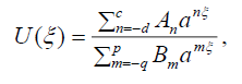
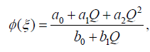
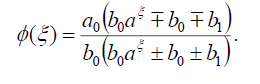
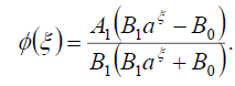
We assume that the formal solution of the ODE (4) can be written in the following rational form:
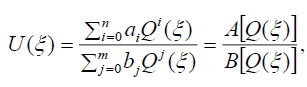 (3)
(3)
where  ,
,  and
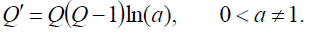
and  . The function Q is the solution of the equation
 (6)
(6)
From (5) and (6), we have
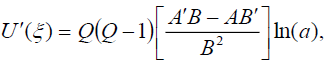 (7)
(7)
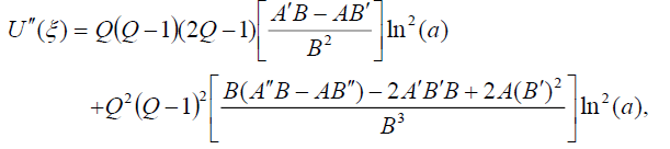 (8)
(8)
and so on.
Step 3
We determine the values m and n in (5) by balancing the highest order nonlinear terms and the highest order derivatives of U(ξ) in Eq. (4) and we can determine a formula of m and n .
Step 4
We substitute (5)-(8) into Eq. (4) and equate all the coefficients of Qi (i = 0,1,2,...) to zero, yield a system of algebraic equations which can be solved using the Mathematica or Maple, to find k ,λ and the coefficients of ai (i = 0,1,...,n) and bj( j = 0,1,...,m). Consequently, we can get the exact solutions of Eq. (2).
The obtained solutions will be depended on the symmetrical hyperbolic Fibonacci functions given in [32,37]. The symmetrical Fibonacci sine, cosine, tangent, and cotangent functions are, respectively, defined as:
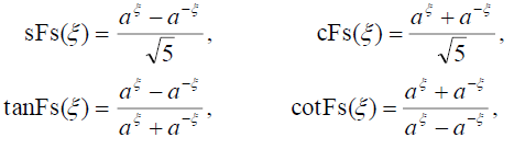 (9)
(9)
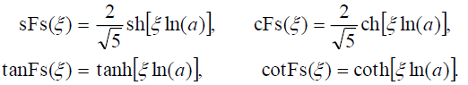 (10)
(10)
Description of the general Expα-function method
With reference to [3] He and Wu have established the well-known exp-function method for solving many nonlinear PDEs. In this section, we give the main steps of the general Expα -function method [32] as follows:
Step 1
We consider (2)-(4) of Sec. 2.
Step 2
According to the general Expα -function method, which was suggested by Ali and Hassan [32], we assume that the wave solution of Eq. (4) can be expressed in the following form:
 (11)
(11)
where p, q, c, d are positive integers to be determined and An ,Bm are constants to be determined too, while 0 < a ≠1 is an arbitrary fixed positive number. We can write (11) in the following equivalent form
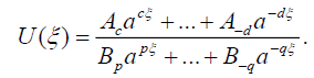 (12)
(12)
Step 3
We determine the values of c, p by balancing the linear term of highest order of Eq. (4) with the highest order nonlinear term. Similarly, we determine the values of d,q by balancing the linear term of lowest order of Eq. (4) with the lowest order nonlinear term.
Step 4
We substitute (12) into Eq. (4) and calculate all the coefficients of ajξ ( j = 0, ±1, ±2, …) Setting all the coefficients to be zero, we get a set of algebraic equations which can be solved by using Maple. Consequently, we can get the exact solutions of Eq. (2).
The obtained solutions will be depended on the symmetrical hyperbolic Fibonacci functions given in (9) and (10).
Applications
In this section, we apply the generalized Kudryashov method and the general Expα -function method describing in sections 2 and 3 to solve Eq. (1) in the following subsections:
On solving Eq. (1) using the generalized Kudryashov method
Let us now solve Eq. (1) using the generalized Kudryashov method. To this aim, we use the wave transformation:
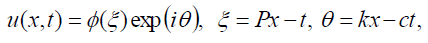 (13)
(13)
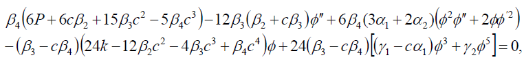
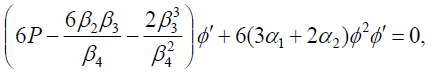
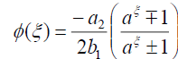
where P, k and c are all constants, while ∅ (ξ ) is a real function of ξ . Substituting (13) into Eq. (1) and separating the real and imaginary parts, we obtain the two ODEs:
 (14)
(14)
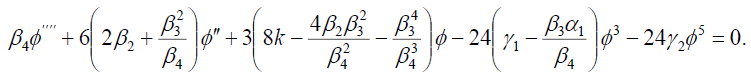
and
 (15)
(15)
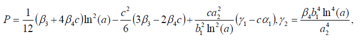
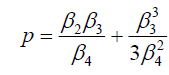
where  ,
,
There are two cases to be considered:
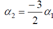
Case 1
If 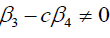 .
.
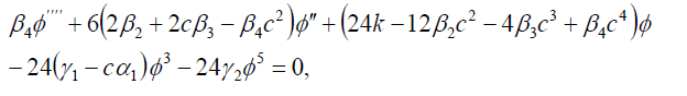
In this case differentiating Eq. (14) and substituting the result into Eq. (15), we have the nonlinear ODE:
 (16)
(16)
Balancing  and
and  in (16), then the following relation is attained:
2(n -m)+ (n -m)+ 2 = 5(n -m) ⇒ n = m+1.
If we choose m =1 and n = 2, then from (5) the formal solution of Eq. (16) has the form:
 (18)
(18)
and consequently,
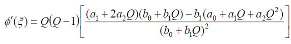 ln(a), (19)
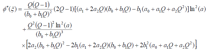 (20)
(20)
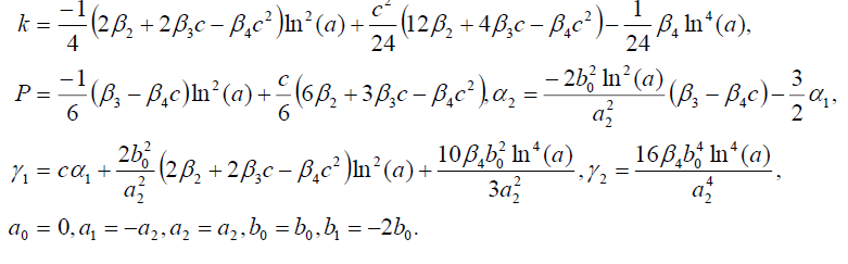
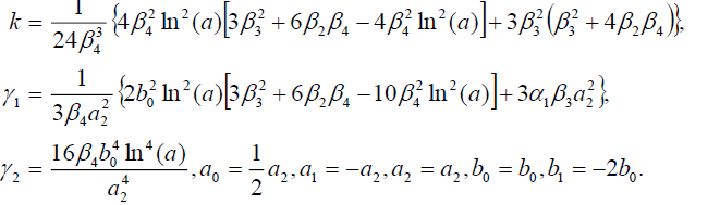
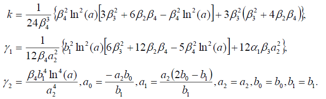
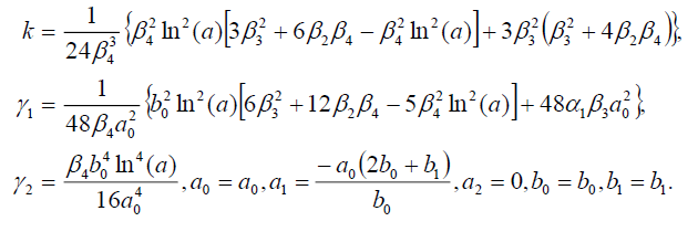
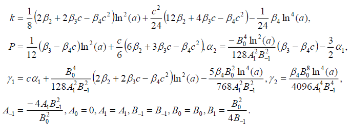
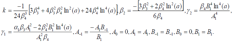
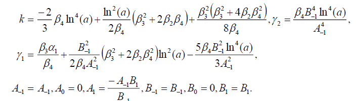
Substituting (18)-(20) into (16), collecting the coefficients of each power of  and setting each of the coefficients to zero, we obtain a system of algebraic equations. Solving this system of algebraic equations with aid of Maple, we obtain the following sets:
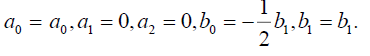
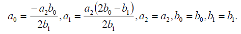
Set 1
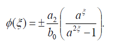
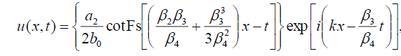
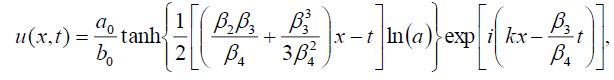
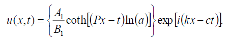
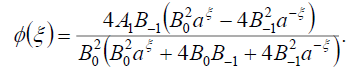
Substituting (21) into (18), we get the following exact solution of Eq. (16):
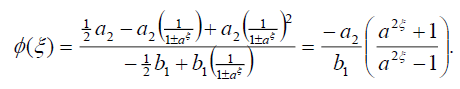 (22)
(22)
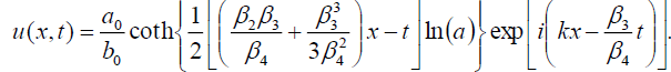
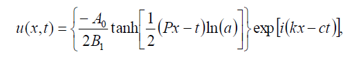
With the help of (9) and (10) the hyperbolic Fibonacci function solution of Eq. (1) has the form:
 (23)
(23)
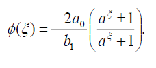
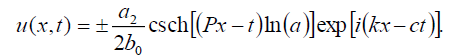
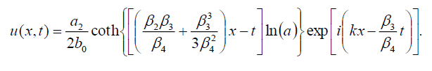
which can be written in the form
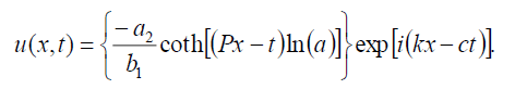 (24)
(24)
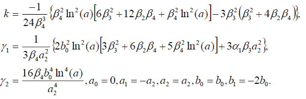
Set 2

 (25)
(25)

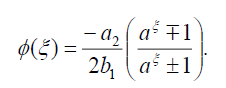
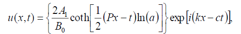
Substituting (25) into (18), we get the following exact solution:
 (26)
(26)
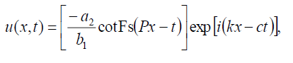
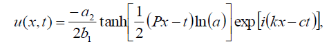
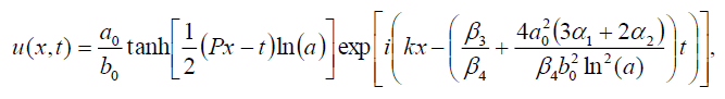
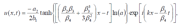
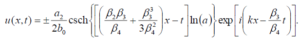
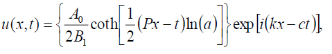
Now, the soliton solutions of Eq. (1) has the form:
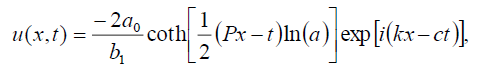 (27)
(27)
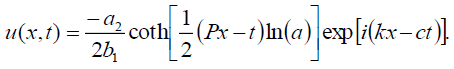
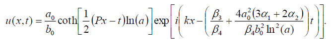
and
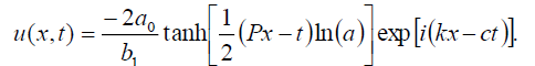 (28)
(28)
Set 3

 (29)
(29)

Substituting (29) into (18), we get the following exact solution:
 (30)
(30)
Now, the soliton solutions of Eq. (1) has the form:
 (31)
(31)
and
 (32)
(32)
Set 4
 (33)
(33)
Substituting (33) into (18), we get the following exact solution:
 (34)
(34)
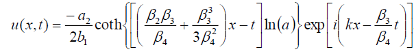
Now, the singular soliton solution of Eq. (1) has the form:
 (35)
(35)
Set 5
 (36)
(36)
Substituting (36) into (18), we get the following exact solution:
 (37)
(37)
If b1 = 0 then we have the soliton solutions of Eq. (1) has the form:
 (38)
(38)
and
 (39)
(39)
Case 2
If  , then we have:
 (40)
(40)
In this case, Eqs. (14) and (15) becomes
 (41)
(41)
and
 (42)
(42)
From Eq. (41), we deduce that:
 ,
,  . (43)
Balancing ø'''' and ø5 in (42), then the following relation is attained:
(n -m)+ 4= 5(n -m)⇒n= m+1.
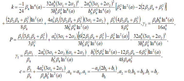
If we choose m =1 and n = 2, then the formal solution of Eq. (42) has the same formal (18). Substituting (18)-(20) into (42), collecting the coefficients of each power of Qi(i = 0,1,...,10) and setting each of the coefficients to zero, we obtain a system of algebraic equations. Solving this system of algebraic equations by the Maple, we obtain the following sets:
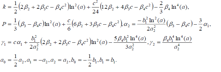
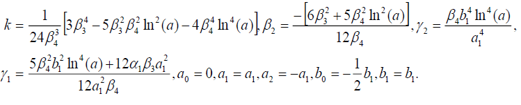
Set 1
 (45)
(45)
Substituting (45) into (18), we get the following exact solution of Eq. (42):
 (46)
(46)
Now, with the help of (9) and (10) the hyperbolic Fibonacci function solution of Eq. (1) has the form:
 (47)
(47)
which can be written in the form
 (48)
(48)
Set 2
 (49)
(49)
Substituting (49) into (18), we get the following exact solution:
 . (50)
Now, the soliton solutions of Eq. (1) has the form:
 (51)
(51)
and
 . (52)
Set 3
 (53)
(53)
Substituting (53) into (18), we get the following exact solution:
 (54)
(54)
Now, the singular soliton solution of Eq. (1) has the form:
 (55)
(55)
Set 4
 (56)
(56)
The result of set 4 follows from the result of set 3 with the interchanges  .
.
Set 5
 (57)
(57)
Substituting (57) into (18), we get the following exact solution:
 . (58)
If b1 = 0 then we have the soliton solutions of Eq. (1) has the form:
 (59)
(59)
and
 (60)
(60)
On solving Eq. (1) using the general Expα -function method
In this subsection, we solve Eq. (1) using the general Expα -function method. To this aim, we use the same transformation (13) to get the two ODEs (14) and (15).
There are two cases to be considered:
Case
If  .
.
In this case, inserting (14) into (15) to get the ODE (16). Let us now determine the positive integers p, q, c, d of Eq. (11). To this aim, we balance the highest order of  and
and  in (16) to get
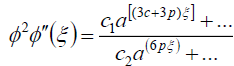 , (61)
and
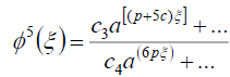 . (62)
where ci (i =1- 4) i are constants. From (61) and (62) we have
3c+3p = p +5c, (63)
which leads to the result
p= c. (64)
In the same way, to determine the values of d, q, we balance the lowest order of and in (16) to get
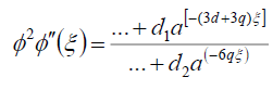 (65)
(65)
and
 , (66)
where di(i =1- 4) i are constants. From (65) and (66) we obtain
-(3d +3q)= -(q +5d), (67)
which leads to the result
q = d. (68)
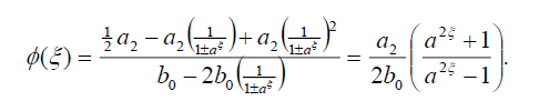
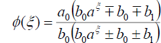
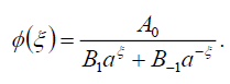
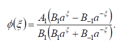
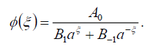
For simplicity, we set p = c =1 and q = d =1. Thus Eq. (16) has the formal solution:
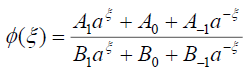 (69)
(69)
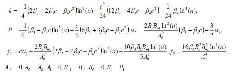
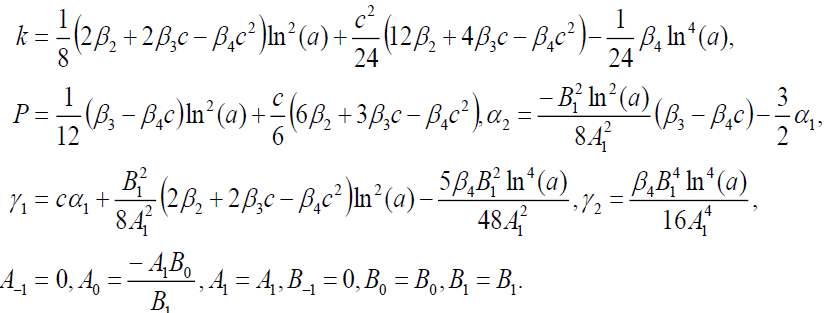
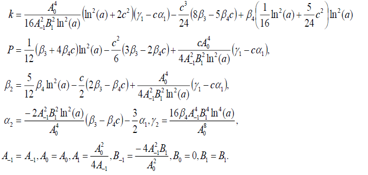
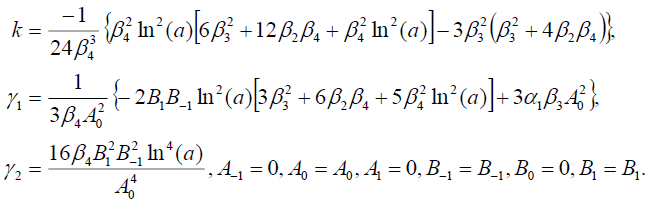
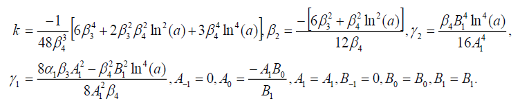
where Ai ,Bi (i = 0,±1) are constants to be determined later. Substituting (69) into Eq. (16) and collecting all the coefficients of ajξ ( j= 0,±1,...,±5) and equating them to zero, we have the set of algebraic equations. Solving these algebraic equations using the aid of Maple, we have the following sets:
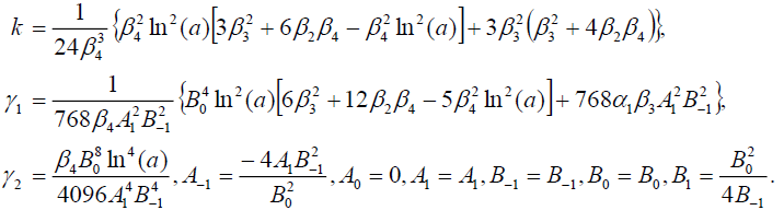
Set 1
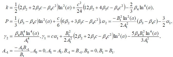 (70)
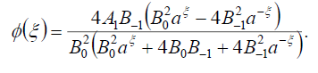
(70)
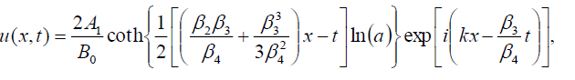
Substituting (70) into (69), we obtain the following exact solution of Eq. (16)
 (71)
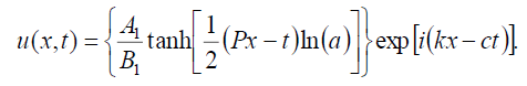
(71)
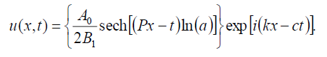
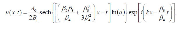
If , B-1 = B1 then with the help of (9) and (10) the hyperbolic Fibonacci function solution of Eq. (1) has the form:
 (72)
(72)
which can be written in the form
 (73)
(73)
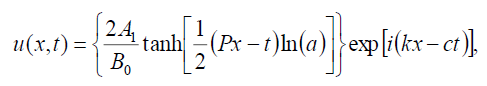
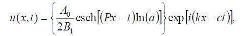
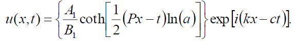
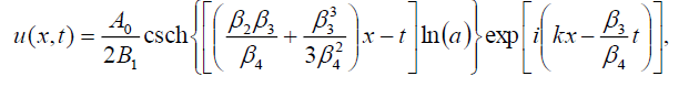
If B-1 = B1 then with the help of (9) and (10) the hyperbolic Fibonacci function solution of Eq. (1) has the form:
 (74)
(74)
which can be written in the form
 (75)
(75)
which is equivalent to the previous singular soliton solution (24) if A1 =-a2, B1 = b1.
Set 2
 (76)
(76)
Substituting (76) into (69), we obtain the following exact solution of Eq. (16)
 (77)
(77)
If  , then the dark soliton solution of Eq. (1) has the form:
 (78)
(78)
which is equivalent to the previous solution (28) if 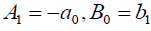 .
.
If , then the singular soliton solution of Eq. (1) has the form:
 (79)
(79)
which is equivalent to the previous singular soliton solution (27) if
Set 3
 (80)
(80)
Substituting (80) into (69), we obtain the following exact solution of Eq. (16)
 (81)
(81)
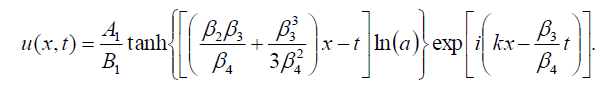
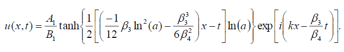
If B-1 = B1 , then the bright soliton solution of Eq. (1) has the form:
 (82)
(82)
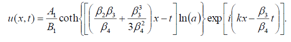
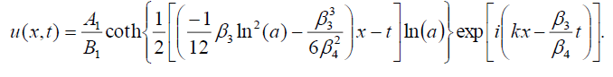
If B-1 = B1, then the singular soliton solution of Eq. (1) has the form:
 (83)
(83)
which is equivalent to the previous singular soliton solution (35) if 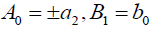 .
.
Set 4
 (84)
(84)
Substituting (84) into (69), we obtain the following exact solution of Eq. (16)
 (85)
(85)
If B0 = B1, then the dark soliton solution of Eq. (1) has the form:
 (86)
(86)
If B0 = -B1, then the singular soliton solution of Eq. (1) has the form:
 (87)
(87)
Set 5
 (88)
(88)
Substituting (88) into (69), we obtain the following exact solution of Eq. (16)
 . (85)
If , then the dark soliton solution of Eq. (1) has the form:
 (90)
(90)
which is equivalent to the previous dark soliton solution (31) if 
If , then the singular soliton solution of Eq. (1) has the form:
 (91)
(91)
which is equivalent to the previous singular soliton solution (32) if
Case 2
If  .
.
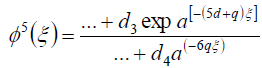
In this case, we use the same steps of case 2 in subsection 4.1 to get the ODE (42). Let us now determine the positive integers p, q, c, d of Eq. (11). To this aim, we balance the highest order of and in (42) to get
 (92)
(92)
and
 (93)
(93)
where ci (i =1- 4) are constants. From (92) and (93) we have
c +15p = 5c +11p, (94)
which leads to the result
p=c
In the same way, to determine the values of d, q, we balance the lowest order of and in (42) to get
 , (96)
and
 (97)
(97)
where di (i =1- 4) i are constants. From (96) and (97) we obtain
-(d +15q)= -(5d +11q), (98)
which leads to the result
q = d. (99)
For simplicity, we set p = c =1 and q = d =1. Thus Eq. (42) has the same formal solution (69). Substituting (69) into Eq. (42) and collecting all the coefficients of ajξ( j = 0,±1,...,±5) and equating them to zero, we have the set of algebraic equations. Solving these algebraic equations using the aid of Maple, we have the following sets:
Set 1
 (100)
(100)
Substituting (100) into (69), we get the following exact solution of Eq. (42):
 (101)
(101)
If B-1 = B1, then the dark soliton solution of Eq. (1) has the form:
 (102)
(102)
If B-1 = B1, then the singular soliton solution of Eq. (1) has the form:
 (103)
(103)
Set 2
 (104)
(104)
The result of set 2 follows from the result of set 1 with the interchanges 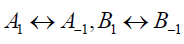 and
and  .
.
Set 3
 (105)
(105)
Substituting (105) into (69), we get the following exact solution of Eq. (42):
 (106)
(106)
If B-1 = B1, then the bright soliton solution of Eq. (1) has the form:
 (107)
(107)
If B-1 = B1, then the singular soliton solution of Eq. (1) has the form:
 (108)
(108)
which is equivalent to the previous singular soliton solution (55) if 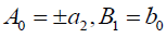 .
.
Set 4
 (109)
(109)
Substituting (109) into (69), we get the following exact solution of Eq. (42):
 (110)
(110)
If , then the dark soliton solution of Eq. (1) has the form:
 (111)
(111)
which is equivalent to the previous dark soliton solution (59) if  .
.
If , then the singular soliton solution of Eq. (1) has the form:
 (112)
(112)
which is equivalent to the previous singular soliton solution (60) if .
Set 5
 (113)
(113)
Substituting (113) into (69), we get the following exact solution of Eq. (42):
 (114)
(114)
If , B0 = B1, then the dark soliton solution of Eq. (1) has the form:
 (115)
(115)
If B0 = -B1, then the singular soliton solution of Eq. (1) has the form:
 (116)
(116)
Some graphical representations of some solutions
In this section, we will illustrate the application of the results established above. Exact solutions of the results describe different nonlinear waves. For the established bright, dark and singular soliton solutions with symmetrical hyperbolic Fibonacci functions are special kinds of solitary waves. Bright, dark and singular soliton solutions have a remarkable property that keeps its identity upon interacting with other.
Let us now examine Figure. 1,2,3 and 4 as it illustrates some of our results obtained in this article. To this end, we select some special values of the obtained parameters, for example, in some of the singular , dark and bright soliton solutions (27), (55), (73) and (107) of the nonlinear Schrödinger equation with fourth-order dispersion and cubic-quintic nonlinearity with a2= b0=b1= A0= A1= B1= c =α1 =β3-1, a = e ,-10 < x, t <10 , respectively.

Figure 1: Plot solution |u(x, t)| of (27) with p =19/6, k =15/4, β2=10/3, β4= 2.

Figure 2: Plot solution |u(x, t)| of (55) with p = 4/3, k = -1/6, β2=β4 =1.
Figure 3: Plot solution |u(x, t)| of (73) with p = 5/6, k =1/4,β2=1,β4 = 2. Figure 4: Plot solution |u(x, t)| of (107) with p = 4/3, k = -1/6, β2=β4 =1. In this article, we have shown that the symmetrical hyperbolic Fibonacci function solutions can be obtained by using the generalized Kudryashov method and the general Expα -function method. As applications, abundant we have obtained many new exact solutions, symmetrical hyperbolic Fibonacci function solutions as well as bright, dark and singular soliton solutions of the nonlinear Schrödinger equation with fourth-order dispersion and cubic-quintic nonlinearity. On comparing our results obtained in this article using these different methods with the well-known results obtained in [34-36] using a different method, we conclude that our results for Eq. (1) are new and not published elsewhere. Further, the different methods used in this article are very powerful and effective techniques in finding the exact solutions, solitary wave solutions and soliton solutions for a wide range of nonlinear problem. Finally, our results obtained in this article have been checked with the aid of the Maple by putting them back into the original Eq. (1).

Conclusion
References