Research

, Volume: 14( 4)

• View PDF
• Download PDF

A Theoretical Model of Space Density: Connecting Electric Charge, Mass, and Internal Energy

Vadim Khoruzhenko*

*Correspondence:

Vadim KhoruzhenkoDepartment of Space Density, Belgorod State University, Belgorod, RussiaE-mail: khoruzhenkova@gmail.com

 

Abstract

My work represents a macroscopic generalization of the Kaluza-Klein theories for quantum systems, concerning the existence of an additional fifth dimension in our space. This allowed Kaluza to unify the descriptions of gravity and electromagnetism within a single mathematical structure. Later, Oskar Klein added a crucial element to Kaluza’s theory by proposing that the fifth dimension is compactified into a very small circle with a radius on the order of the Planck length. Due to its minuteness, this dimension remains invisible at ordinary scales. Additionally, I drew upon ideas proposed by Feynman, who suggested using the concept of energy density in space to describe electromagnetic interactions at the quantum level within the framework of Quantum Electrodynamics (QED). This theory helps explain how, at short distances, charge screening and renormalization occur due to interactions with virtual particles in the vacuum. In my work, I attempt to describe the observable effects at the macroscopic level, such as the electric interaction of charges and the gravitational interaction of massive bodies, through an intuitively understandable process of spatial disturbance. This disturbance is first expressed in the disruption of the uniform distribution of spatial density and then in the curvature of the spherically symmetric structure of the disturbance. In formulating my theory at a macroscopic level, which implies a statistical averaging of the processes described by Kaluza, Klein, and Feynman at the quantum level, I was primarily inspired by the ideas proposed by these scientists. I aimed to formalize their mathematical concepts into simple and intuitively understandable postulates, which lead to observable effects in macro-objects. One such effect is the attenuation of the electric field at short distances between charges, similar to the processes occurring at the quantum level. Based on innovative theoretical insights, this work provides yet another alternative confirmation of the Theory of Relativity regarding the equivalence of energy and mass of elementary particles.

 

Keywords

Finitely distinguishable independent features hypothesis; Higher-order moment convergence; Vlasov-Fokker-Planck equation; Kinetic moment-closed model; Fokker-Planck-Rosenbluth collision operator; Axisymmetry

Introduction

Electromagnetic and gravitational forces are among the most fundamental interactions known to physics. These forces govern the behavior of matter and energy across scales, from subatomic particles to the cosmos. Despite extensive empirical data and theoretical models describing the behavior of these forces, their true nature and the material essence from which they arise remain subjects of deep inquiry.

From a physical standpoint, we understand how these forces act and can accurately predict their effects. However, questions remain: what exactly are these forces? How are they interconnected? And, most importantly, what is the proto-matter, the fundamental substance from which these forces emerge? These questions touch not only on physical principles but also on philosophical reflections about the nature of reality.

In this paper, we propose a theoretical model that introduces a fifth spatial dimension, referred to as” space density.” We hypothesize that this dimension plays a critical role in the formation of gravitational and electric fields. Us model suggests that the traditional three-dimensional space, combined with time, is insufficient to fully explain the origin of these forces. Instead, space itself may possess internal properties that contribute to the formation of these fields. By expanding our understanding of space to include an additional dimension, we explore the potential for new interpretations of gravitational and electromagnetic interactions.

Hypothesis

We hypothesize that electromagnetic and gravitational fields are manifestations of a more fundamental property of space, which we call” space density.” This property is defined in a five-dimensional system, where the fifth dimension is orthogonal to the traditional three spatial and one temporal dimensions.

In this model, “space density” represents a measure of how space itself can be compressed or expanded independently of its metric. This density is not analogous to the density of matter with which we are familiar in three-dimensional space, but rather reflects a fundamental characteristic of space that influences the formation of gravitational and electric fields.

Our hypothesis is based on several key postulates:

Space density: In five-dimensional space, the density ρ(r) characterizes the state of space and can vary, allowing us to describethe curvature of space without distorting its metric. Let us call this phenomenon first- order space curvature. A similar term isused in the theory of relativity, but in this theory, it will have a slightly different context.

Spherical symmetry of disturbances: The distribution of space density under disturbance assumes spherical symmetry. Thedistribution of space density ρ(r) is assumed to be symmetric relative to the point that is the center of disturbance.

Conservation of space density: When a region of space is disturbed, the surrounding space is capable of changing its densityin such a way that the total density of the entire space remains constant. In other words, in a certain approximation, we can saythat the total “density” of space over a finite volume much larger than the volume of the disturbance should remain constant.

Minimization of entropy: Space tends to states of minimum entropy relative to the distribution of space density. This principlegoverns the natural tendency of space to return to a uniform density distribution after disturbances, similar to the thermodynamicprinciples that govern physical systems.

By exploring these postulates within the framework of five-dimensional space, we aim to provide a deeper understanding of the origins of gravitational and electromagnetic fields. This model challenges the traditional notion that these fields are independent and instead suggests that they are interconnected through the intrinsic properties of space itself.

Materials and Methods

Distribution of space density around a compressed spherical region of space

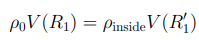
We have two states of the universe. In the first state, the density throughout space is ρ0 and is a constant. In the second state of the system, there is a region of space bounded by a sphere S(R1), which we compress to S (R1′). We need to find the distribution of space density inside and outside the sphere, based on the laws we have established in our hypothetical universe.

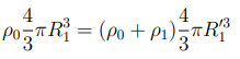
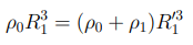
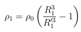
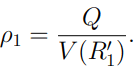
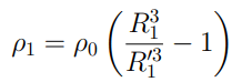
Density distribution after compression: The density after compression inside the sphere is given by ρinside=ρ0+ρ1, where ρ1 is the added density, determined by the ratio of the volumes before and after compression:

Substitute the volumes of the spheres:

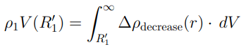
Simplifying:

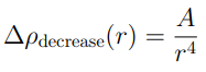
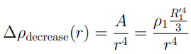
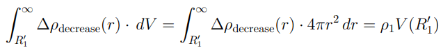
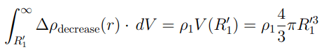
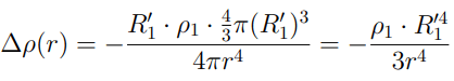
Density distribution outside the sphere: We assume that outside the sphere, the amount of extracted space density must equal the amount added inside it, ρ1V(R1′). Therefore, when integrating the disturbance from the surface of the compressed sphere to infinity, the integral must converge to a finite number, meaning the integrand must be convergent. In three-dimensional space, such a function is 1/r4. Let us assume that the distribution of reduced density outside the compressed region of space will follow this distance dependence from the center of disturbance. Thus, we get the following dependence for the space density distribution outside the compressed sphere:

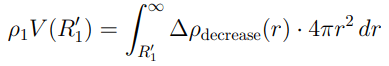
Normalization coefficient A: To satisfy the law of conservation of space density, the integral of Δρdecrease(r) over the volume from R1′ to infinity must equal the added density inside the sphere:

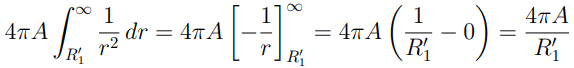
Considering the law of spherical symmetry, in spherical coordinates, the integral simplifies to:

Substituting:

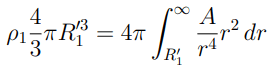
Solve the integral:

The equality of densities:

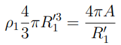
Find A:

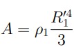
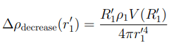
The final formula for Δρdecrease(r):

Now multiply both the numerator and denominator by 4π:

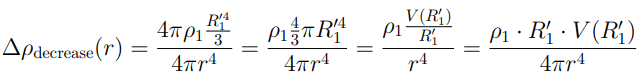
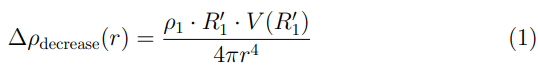
Thus, we have derived the following formula for the density distribution outside the sphere Δρdecrease(r):

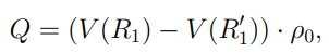
Considering that the amount of added density in the volume of the compressed sphere is expressed by the formula:

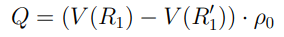
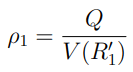
where V(R1) and V(R1′) are the volumes of the spheres with radii R1 and R1′, respectively. Also, taking into account the formula for ρ1 the density of the added density inside the sphere:

where V (R1′) is the volume of the sphere after compression. We can express the derived formula for the space density distribution Δρdecrease(r) as:

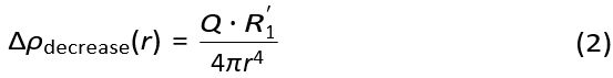
Where Q is the amount of density added to the volume of the sphere S(R1′), R1′ is the radius of the compressed sphere, and r is the distance from the center of the sphere to the point in space in spherical coordinates.

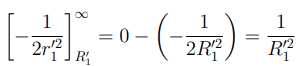
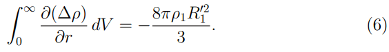
Verification of space density conservation: To satisfy the third law established in our system, the following equality must hold:

Substitute the expression for Δρdecrease(r):

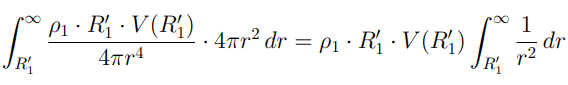
Integrate and apply the limits

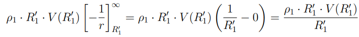
We get:

Thus, we have confirmed that our space density distribution outside the compressed sphere, proportional to 1/r4, agrees with our third law of space density conservation in the system, taking into account the normalization coefficient A.

Interaction of two compressed spheres of space

In this section, we explore the interaction between two compressed spherical regions of space. By analyzing the distribution of space density around these spheres, we derive the influence of one sphere on the density distribution of the other. This analysis is crucial for understanding the nature of forces and interactions that arise due to variations in space density.

Illustration of space density distribution

Before proceeding with the mathematical derivations of the impact of space density distribution created by two spheres on each other, I suggest examining a graphical representation of the space density distribution around two compressed spheres. This figure, constructed based on the mathematical model using the formula derived for Δρdecrease(r) (Equation 2), visually demonstrates how the density distribution created by each sphere changes depending on the distance between them (Figure 1).

FIG. 1. Space density distribution around two compressed spheres. The graph illustrates how the space density changes along the line connecting the centers of the spheres as they approach each other.

Integral of the density gradient for one sphere

Consider the function Δρdecrease(r1′), which represents the density distribution for one sphere and has spherical symmetry with respect to the coordinate system r1′. The function takes the form:

where R′1 is the radius of the sphere, ρ1 is the density at radius R′1, and V (R′1) is the volume-dependent function.

Gradient of the density function in the r1′ coordinate system: I propose that the amount of disturbance created by the second sphere on the space density distribution of the first sphere can be described by calculating the integral of the gradient of the space density distribution outside the spheres in a coordinate system centered at the first sphere. Accordingly, to calculate the influence of the first sphere on the second, the same process should be applied, but in the coordinate system centered at the second sphere. Let us verify the outcome of such assumptions.

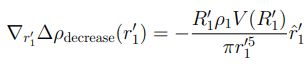
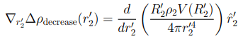
First, we compute the gradient of the function Δρdecrease (r1′) with respect to the radial coordinate r1′. The gradient operator in spherical coordinates for a radially symmetric function is given by:

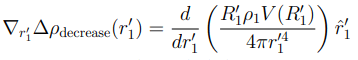
Where rˆ1′ is the unit vector in the radial direction. Taking into account the spherical symmetry, we compute the derivative with respect to r1′ and obtain:

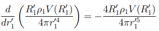
Thus, the gradient of the density function in spherical coordinates r1′

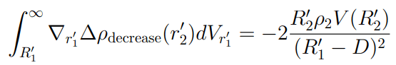
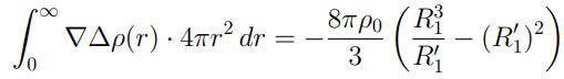
Integral of the Gradient from R1′ to Infinity Next, we integrate the gradient of the density function from R1′ to infinity:

where dVr1′ = 4πr′12dr′1 is the volume element in spherical coordinates r1′. Substituting the previously obtained gradient:

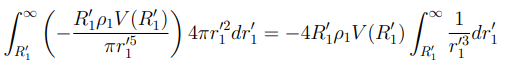
Solving the integral:

Substituting the integration limits from R1′ to infinity, we get:

Finally, substituting this into the integral

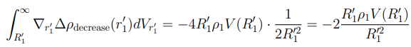
Simplifying the expression:

Integral of the density gradient for the second sphere

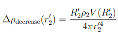
Consider the density distribution for the second sphere Δρdecrease (r2′), which is spherically symmetric with respect to the coordinate system r2′. The function is given by:

Considering the invariance of the position of the second sphere relative to the first in the coordinate system r1′ at a fixed distance D (the system of two spheres is invariant to the coordinates of the center of the second sphere in the r1′ coordinate system and depends only on the distance D), the relationship between the radius vectors in the two reference systems can be expressed as: r2′= r1′−D, where D is the fixed distance between the origins of the coordinate systems r1′ and r2′, respectively.

Gradient of the density function in the r1′ coordinate system: Having the relationship between the radius vectors of the coordinate systems r1′ and r2′ to compute the gradient of Δρdecrease(r2′) with respect to r1′, it is necessary to apply the chain rule. The gradient of the function Δρdecrease (r2′) with respect to r2′ is given by:

Using the chain rule, we get:

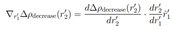
Where dr′2/dr′1=d/dr′1 (r1′—D)=1, since D is a constant value.

Thus, the gradient of Δρdecrease (r2′) in the r1′coordinate system is:

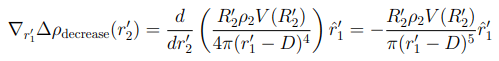
Application of the change of variables theorem: To perform the integration, we apply the change of variables theorem. Considering that r2′= r1′—D, we find that r1′=r2′+D.

Verification of the chain rule application: The chain rule can be applied since the function Δρdecrease (r2′) is continuously differentiable with respect to r2′. Moreover, the relationship between r1′ and r2′ is linear, ensuring that the condition dr1′/dr2=1 is satisfied.

Verification of the change of variables theorem: To apply the change of variables theorem, the following conditions must be verified:

Continuity of the transformation: The transformation r2′=r1′−D is continuous and differentiable.

Jacobian calculation: The Jacobian of the transformation r1′= r2′+D equals dr1′/ dr2′=1.

Transformation of integration limits: The integration limits are transformed as follows:

Lower limit: r1′=R1′ corresponds to r2′=R1′—D.

Upper limit: r1′=∞ corresponds to r2′=∞.

Thus, the change of variables theorem is applicable, and the integral in the r2′ coordinate system is:

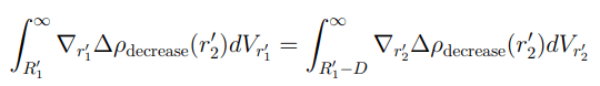
Integral of the gradient in the r2′ coordinate system: Now, let’s integrate the gradient of the density function Δρdecrease (r2′) over the volume element dVr′2=4πr′22dr′2

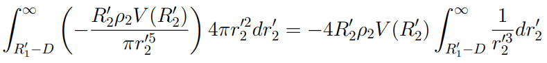
The integral simplifies to:

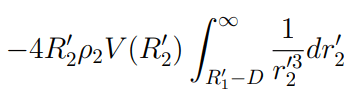
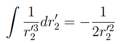
Solving the integral:

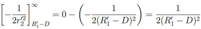
Integrating from R1′—D to infinity, we get:

Thus, the integral of the gradient of the function Δρdecrease(r′2) in the r′1 coordinate system is:

Disturbance of the density distribution of the first sphere in the presence of the second sphere

Determination of the disturbance magnitude: I propose that the disturbance of the density distribution of the first sphere in the presence of the second sphere, located at a distance D, is determined as the difference between the integral of the gradient of the total density distribution for the two spheres in the r1′ system and the integral of the gradient of the density distribution for one sphere, also in the r1′system.

This disturbance represents the “amount of influence” of the second sphere on the density distribution of the first sphere. I also hypothesize that the amount of disturbance, according to the fourth postulate of our system, will equal the amount of “interaction” between the systems. Space, striving to minimize its entropy, will” affect” the spheres by changing their position in space, thereby reducing the disturbance.

Mathematically, the disturbance magnitude ΔWr1′ (D) is defined as:

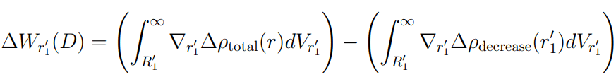
where:

is the total space density distribution created by the two spheres in the r1′ coordinate system, while:

Is the density distribution created by the first sphere, again in the r1′ coordinate system?

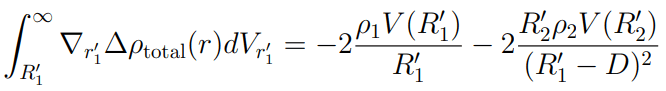
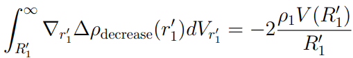
Now, the disturbance magnitude ΔWr1′ (D)—the amount of disturbance in the space density created by the second sphere on the space density distribution of the first sphere in the r1′coordinate system—can be computed as the difference between these two integrals

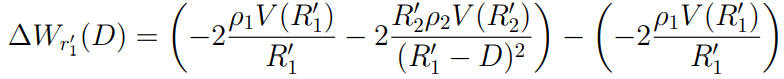
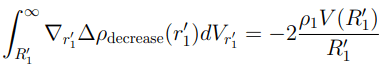
Simplifying the expression:

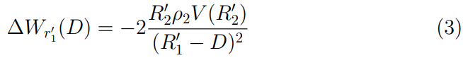
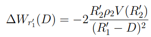
Approximation for large distances D?R1′: In the approximation where D?R1′, the formula for the disturbance simplifies and becomes similar to the expression for the electric field intensity created by a point charge. Specifically, the magnitude ρ2.V(R1′) can be interpreted as the equivalent of the electric charge Q of the second sphere, representing the added space density of the second sphere in the volume V (R1′).

The radius R1′ in the numerator acts as a normalizing constant, and D represents the distance between the centers of the spheres S(R1′) and S(R2′), where the added space density is concentrated, which can be analogous to electric charges. With this analogy in mind, the disturbance magnitude ΔWr1′ (D) for large distances can be expressed as:

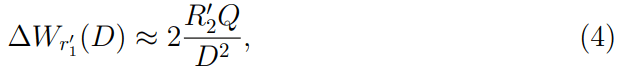
where Q=ρ2V (R2′), or Q= (V (R2) − V (R2′)) ·ρ0

This formula highlights the direct proportionality of the disturbance ΔWr1′ (D) to Q and the inverse-square dependence on the distance D between the “charges,” which is characteristic of fields such as the electric field created by point charges. Given the similarity of the obtained formula to the formula for the electric field intensity, in our interpretation, Q takes on the physical meaning of charge, and ΔWr1′ (D) takes on the physical meaning of electric field intensity or the force exerted by the charge Q on a unit charge located at a distance D. This result is very important for our theory, as it gives us confidence that our hypothetical assumptions about the nature of space are likely correct, and our theory transitions from an abstract model to having practical significance in understanding the origin of such phenomena as charge and the electric field.

Physical interpretation: Given the similarity of this disturbance formula to the formula for the electric field intensity derived from Coulomb’s law, which was originally obtained based on experimental data, it can be reasonably assumed that our assumptions about the properties of space density in the context of real physical phenomena, such as the electric field, are correct. This analogy provides a conceptual bridge between the abstract mathematical formulation of space density disturbance and well-known physical laws governing electric fields.

Thus, the presence of the second sphere at a distance D leads to a disturbance in the space density distribution of the first sphere,similar to the influence of a point charge on the electric field at a distance. This connection not only confirms the validity of our theoretical approach but also provides a deeper understanding of the interaction between space density distributions and their physical interpretations.

Results and Discussion

The results obtained from the analysis of the interaction between two compressed spheres suggest a profound connection between the concepts of space density and classical field theories. The derived formula for the interaction of space density disturbances bears a striking resemblance to Coulomb’s law for electric fields, implying that what we understand as electric charge may be deeply rooted in the fundamental properties of space.

This similarity opens up new perspectives for interpreting the nature of electric and gravitational fields, suggesting that these fields are not merely byproducts of the presence of matter, but are intrinsic to the very fabric of space itself. The hypothesis that space can possess a “density” that influences the formation of fields challenges traditional views of space as a passive backdrop for physical phenomena.

The presented mathematical model provides a new foundation for understanding the forces that govern the universe. The introduction of the concept of a fifth dimension gives us a new perspective on the interaction of forces, potentially leading to a unified theory encompassing both gravitational and electromagnetic interactions.

The potential implications of this model are vast. If the connection between space density and the formation of fields is confirmed by further theoretical and experimental work, it could lead to a reevaluation of fundamental concepts in physics. This model may offer new insights into the unification of forces, the nature of dark matter and dark energy, and the role of additional dimensions in the structure of the universe.

Future research should explore the broader applicability of this model, including its implications for quantum field theory, cosmology, and high-energy physics. Additionally, experimental verification of the predicted space density distributions and their effects on observable phenomena will be critical to confirm this theory. The introduction of space density as a fundamental property of space itself opens new avenues for both theoretical and experimental research.

Solving the gradient integral over the entire volume for the space density distribution equation of one sphere

In this section, we solve the gradient integral over the entire volume for the space density distribution equation of one sphere. The approach uses the Heaviside function, which effectively describes boundary conditions and sharp transitions in the space density distribution. This detailed derivation ensures the conservation laws are upheld and provides insight into the nature of space density disturbances.

We will write our distribution taking into account the boundary conditions using the Heaviside function and integrate the gradient of this space density distribution over the entire volume. The idea is that mass, in the classical sense of mass, is also related to space density. The curvature of space, along with its metric (second-order curvature) and the curvature of space relative to its metric (first-order curvature), such as the change in space density distribution different from the uniform distribution ρ0, is inevitably tied to boundary conditions! Based on the postulates of our space, according to the fourth postulate of our space, the space density inside the compressed sphere will always be homogeneous, while at the boundary of the sphere, there will always be a sharp transition in density, which can be described by the Heaviside function. Thus, to again satisfy the fourth postulate of our space the tendency to minimize entropy space will tend to curve further. I hypothesize that it is precisely the boundary conditions, such as the discontinuity in the uniform distribution of space density, which is undoubtedly a strong space density disturbance, that cause the curvature of space along with its metric. Below is an illustration showing the space density distribution along any radial vector from the center of the disturbance to infinity (Figure 2).

FIG. 2. Graphs of space density distribution along a line passing through the center of the compressed sphere.

Representation of space density distribution using the Heaviside function

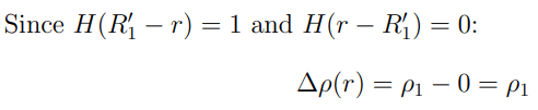
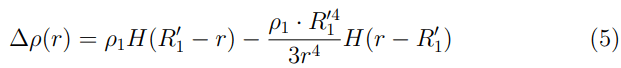
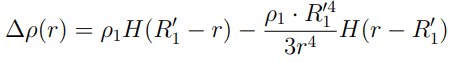
The space density distribution, ρ(r), for a single sphere can be expressed using the Heaviside function H(x) for an accurate description of the density inside and outside the compressed sphere. The primary density distribution is defined as:

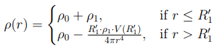
The increase in density Δρincrease(r) within the compressed region can be expressed as:

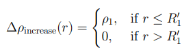
Similarly, the decrease in density Δρdecrease(r) outside the sphere is:

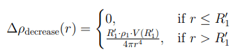
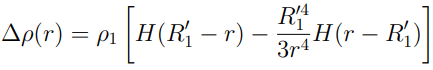
Now we can rewrite these expressions in terms of the Heaviside function H(x):

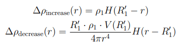
Thus, the overall change in density Δρ(r):

Boundary condition verification

Now let’s verify the boundary conditions:

For r ≤ R′1:

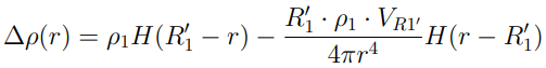
For r>R′1:

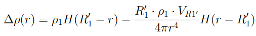
Now substitute VR1′=4/3π(R′1)3:

Thus, we arrive at the following expression for Δρ(r) in terms of the Heaviside function:

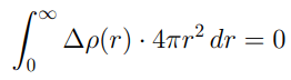
Verification of the space density conservation equation

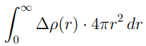
To verify, we will take the integral of Δρ(r). Let’s integrate Δρ(r) over the entire volume. Recall that Δρ(r) is given by:

We will calculate the integral:

We divide the integral into two parts, corresponding to Δρincrease(r) and Δρdecrease(r):

We split this into two separate integrals

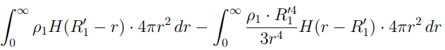
Let’s first consider the first integral:

Now consider the second integral

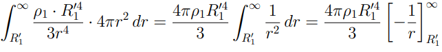
We evaluate the limits:

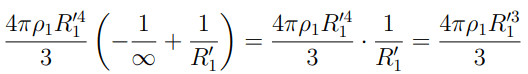
Now let’s add both results:

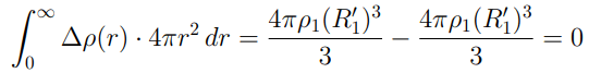
Thus, the integral of Δρ(r) over the entire volume equals zero:

We obtained the expected result, though this calculation was necessary for verification.

Calculation of the gradient integral and verification of the fourth law of our system

In this section, we will calculate the integral of the gradient of the space density distribution over the entire volume, written in terms of the Heaviside function, to determine whether space is in a disturbed or equilibrium state. In other words, since we established in the previous section that the gradient integral of the space density distribution has the physical meaning of a force, let us find the expression for the force that keeps our space in a compressed state inside the sphere S(R1). Now we will focus on calculating the gradient and subsequently integrating it from the function ∇Δρ(r), expressed using the Heaviside function.

In the previous subsection, we obtained the following space density distribution for a single sphere Δρ(r):

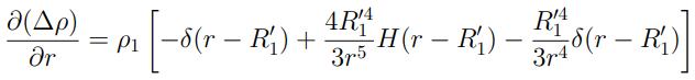
Calculation of the gradient over the volume from the obtained space density distribution for one sphere ∇Δρ(r):

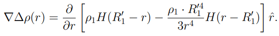
Let’s find the gradient ∇Δρ(r):

Derivative of H(R1′−r):

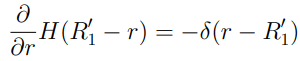
Derivative of R′4/3r4 H(r−R′1) is:

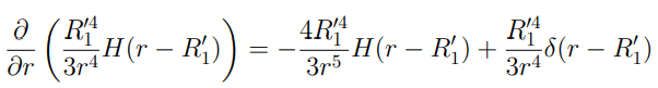
The final partial derivative is:

Now let’s compute the integral of the gradient over the entire volume from ∇Δρ(r), which is:

Our expression for the gradient integral takes the form:

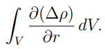
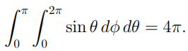
In spherical coordinates, the volume element dV is equal to r2 sin θ dr dθ d?. Since the function ∂(Δρ)/∂r depends only on the radial coordinate r, the angular integrals can be computed separately:

Thus, the integral simplifies to:

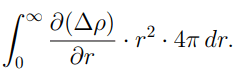
Now substitute the function ∂(Δρ)/∂r:

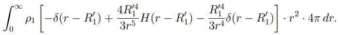
We divide the integral into three parts:

Now we compute each integral part:

Integral of –δ (r − R1′)· r2

Using the property of the delta function:

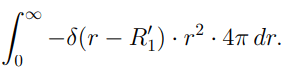
The delta function property states:

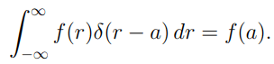
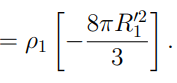
Here, f (r)=−r2· 4π and a=R1′. Thus:

Integral of 4R′41/3r5 H (r−R′1)· r2

For the function H(r−R1′), the integral is limited from to R1′ infinity:

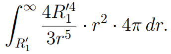
We simplify the integrand:

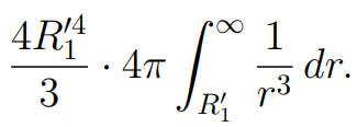
The integral over r:

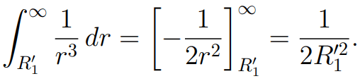
Thus:

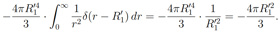
Integral of -R′14/3r4 δ(r−R′1)· r2

Using the property of the delta function:

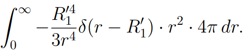
The delta function allows us to simplify this integral:

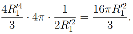
Now let’s sum all the parts:

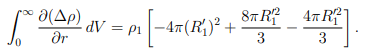
Combining the results:

We get:

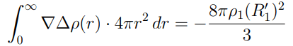
Thus, the final result of the integral is:

Expressing the result through the area of the sphere S(R1′):

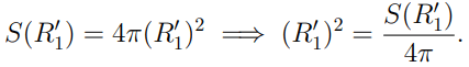
Substituting into the integral:

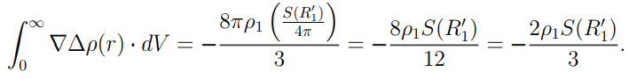
Thus, the gradient integral over the entire volume in terms of the sphere’s area S(R1′) is:

Now let’s express the result through Q, considering that:

Where Q is the amount of added density to the volume bounded by the sphere S(R1′) and is expressed by the formula:

and V(R1) and V (R1′) are the volumes of the spheres with radii R1 and R1′, respectively. We get the formula for the disturbance of space density caused by a single compressed sphere:

We obtained the same dimensionality as the formula for ΔWr1′(D)≈2R2′Q/D2, if we cancel out R′2 and the square from D2, we get the same dimensionality as the electric field intensity, which characterizes the force with which the electric field intensity acts on a unit electric charge at a distance D between the centers of the spheres. This means that our reasoning was correct; the integral of the gradient for the space density distribution from 0 to infinity indicates the force required to keep the space density in a compressed state.

We also see that, despite the fulfillment of the third postulate of our system the law of conservation of space density the system is not in equilibrium and remains disturbed. Thus, to satisfy the fourth law of our universe the tendency to minimize the entropy of the space density distribution the amount of space density disturbance must also tend to zero. How- ever, if we make further changes to the space density distribution outside the sphere and somehow redistribute the space density outside the sphere, this will violate the third law associated with the conservation of space density.

In this regard, it can be assumed that space, in order to compensate for this disturbance, will curve along with its metric. In this way, both the third and fourth postulates of our hypothetical universe will be observed. Now we need to find such a space density distribution that will lead to zero disturbance of space density caused by the boundary conditions on the compressed sphere.

Conclusions on the gradient integral

The integration of the space density gradient over the entire volume yielded a significant result that confirms the hypothesis that space density plays a key role in the formation of gravitational and electromagnetic fields. The non-zero result of the gradient integral, with a negative sign, indicates that the system is in a disturbed state and requires further changes to achieve equilibrium.

This disturbance can be interpreted as space curvature, which is directly related to changes in the space density distribution caused by the compression of a spherical region. The result obtained suggests that space curvature and space density disturbances are closely linked, providing new insights into the nature of gravitational interactions.

Additionally, the expression obtained for the total disturbance highlights the relationship between the three-dimensional surface area, space density, and the resulting disturbance. This relationship points to a deeper connection between space density and the forces that govern the behavior of matter and energy in the universe.

The introduction of the concept of space density as a fundamental property of space itself, capable of influencing the distribution and interaction of fields, opens new avenues for understanding the fundamental forces of nature. This theoretical framework offers the potential to unify gravitational and electromagnetic phenomena under a common conceptual basis, which could lead to new discoveries about the nature of matter, energy, and the structure of the universe.

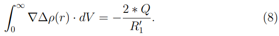
The relationship between space density and the mass of a compressed sphere

In the previous section, we obtained that ∫∞0 ∇Δρ(r)·dV=−2∗Q/R1′, which is non-zero and characterizes the force that keeps the sphere with space density compressed.

Now, let’s calculate the energy required to compress this sphere from S(R1) to S(R1′). If the integral of the gradient is a measure of force, then by integrating this force along the path, we will obtain the work necessary to compress the sphere, i.e., its internal energy.

Next, we will find this relationship between the internal energy of the charge, equal to the integral of the force required to compress the sphere, over the radius from its initial radius R1 to the final radius R1′. This relationship is crucial for understanding how the energy contained within the compressed sphere determines the curvature of space, and consequently, the gravitational field generated by the compressed region of space in the form of a sphere, i.e., its mass.

Energy required to compress the sphere from R1 to R1′

Initial equation

We have:

where

Substitute the value of ρ1 and get:

Let’s perform a variable substitution, replacing R1′ with t, so that our expression takes the form:

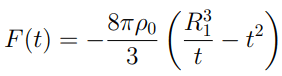
Here, F (t) represents the physical force required to compress the sphere S(t) from t′=R1 to t′=R1′.

Calculating the energy required to compress the sphere from R1 to R1′

Consider the sphere S(t) with radius t, which needs to be compressed from radius R1 to radius R1′. The force that holds the sphere in a compressed state S(R1′) is given by the function:

We need to find the energy E, expended in compressing the sphere from R1 to R1′. To do this, we use the formula for work, which in this case is equal to the compression energy:

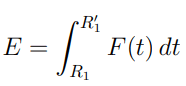
Substitute the expression for force F (t):

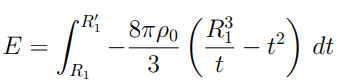
We split the integral into two terms:

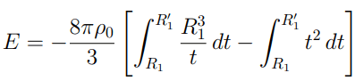
Integrating each term with respect to t:

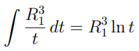
For the first term, we get:

For the second term, we get:

Substitute the integration results and limits of integration:

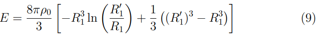
This expression represents the energy required to compress the sphere from R1 to R1′. This energy is equivalent to the amount of energy contained within the compressed sphere, which causes the curvature of space along with its metric, thereby determining the mass of the sphere.

Mass of the compressed sphere

Using the well-known Einstein equation E=mc2, we can find the mass m of the compressed sphere:

This expression defines the mass of the compressed sphere based on the energy required for its compression, which can also be interpreted as the energy that holds the sphere in a compressed state or the energy contained within the compressed sphere. This result illustrates how the energy associated with compressing the sphere is converted into equivalent mass, which (in accordance with our fourth postulate) creates the curvature of space relative to its metric and gives rise to effects such as mass and the gravitational field.

Transition to gravitational equations

The obtained value of the energy required to compress the space density sphere is nothing more than the energy required to create this clump of space density. One could say that this is the internal energy of the electric charge or the gravitational charge; the essence remains the same. According to the fourth law of our system, space will strive to reach equilibrium and curve the metric of space, thereby fulfilling the fourth postulate of minimizing the entropy of space energy and bringing the system to equilibrium.

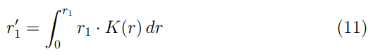
We can, similarly to the calculation of first-order curvature characterized by Δρdecrease(r), obtain the curvature coefficient K(r), which represents the coefficient of curvature of the space metric at each point in space created by the energy clump E, as per Formula No. 9.

Unlike first-order curvature, which is characterized by the electric field, the transition between first-order space r1 and second-order space r1′ relative to which our space will be curved will follow the following relationship for the radial vectors:

Thus, unlike electric fields, whose values combine and form a new field distribution upon interaction, the curvatures caused by energy clumps E will multiply. This also defines the nature of the interaction, in contrast to the interaction of electric charges. Energy objects, or as we commonly under- stand them, massive bodies, will distort the curvature distributions created by other objects not by adding the curvature coefficients but by multiplying them, unlike how we did with the analogs of our electric charges S(R1′) and S(R2′). Therefore, at short distances comparable to the sizes of massive bodies, to minimize the amount of mutual curvature and entropy of space, energy objects (or simply, bodies with mass) will attract each other. At larger distances, when the coefficient of mutual curvature of space metrics is small, they will repel each other with acceleration, similar to electric charges. This explains phenomena such as dark matter and dark energy.

The curvature of the spatial metric K(r), similar to the distribution of density outside the compressed sphere, will be proportional to 1/r4 with an appropriate normalization coefficient. This coefficient K(r) describes the distribution of space-time curvature caused by the energy clump and allows us to establish an equation for this distribution.

Next, we will need to consider the perturbations caused by a second gravitational charge on the distribution of the coefficient K(r) in the coordinate system of the first one, describing the curvature of the space-time metric due to the first charge, similarly to how we did with electric charges, except that the curvature coefficients from two bodies do not add but multiply, to create a unified picture of the gravitational field generated by two energy objects, or as we commonly call them, bodies with mass. This mutual perturbation and its influence on the curvature of space up to the second body will lead us to equations similar to gravitational equations, but more precise, which will account for the repulsion of massive bodies at large distances.

This simple explanation covers concepts such as energy, charge, electric field, mass, gravitational field, dark matter, and dark energy. The space density that we introduced at the beginning of our study as a hypothetical value has a physical dimensionality equal to a coulomb divided by a unit of volume. In turn, the charge is the difference in the volumes of spheres before and after compression, multiplied by the space density in the state of minimal entropy, ρ0.

Physical meaning

The calculations performed serve as further confirmation of the theory of relativity, which asserts the equivalence of energy and mass. What we understand by mass, as a measure of matter that manifests itself in gravitational effects through the curvature of the space metric, is nothing more than the amount of energy spent on compressing the space density from the sphere S(R1) to S(R1′), where R1′

Thus, this creates an analogy opposite to the first case of electric charge: If the first case is taken as a negative charge, then the second would correspond to a positive one. It should also be noted that the amount of energy required to stretch the space density with the same charge will be greater, and the “geometric” size of the stretched sphere will also be larger, which relates us to elementary particles electrons and protons and the ratio of their masses and sizes with identical electric charges. Undoubtedly, the representation of charges as spheres is an approximation, and in reality, we do not yet know the geometric structure of elementary charges, and their mass-to-size ratio will depend on this geometric structure.

The proposed approach to the relationship between the mass and size of elementary charges allows us to analyze possible geometric structures of elements of the micro-world. However, already knowing the mass of the electron and the proton, we can approximately calculate the ratio of S(R1) to S(R1′) that satisfies the observed mass ratio of electrons and protons. Thus, we can already obtain calculated data for the relative ratio of the compression coefficient K=R1/R1 of the space density necessary for the formation of elementary particles. Next, using our formula for the amount of energy in the space density, we can determine the internal energy of an elementary particle in units of ρ0. Knowing the internal energy, we can also calculate the value of ρ0, which will allow us to express all known physical quantities in terms of units of measurement of ρ0, the dimensionality of which is coulomb divided by unit volume.

Calculation of the electric field based on the macroscopic space density model for distances between charges com- parable to the size of the charges: Renormalization and screening of charges

To demonstrate the effectiveness of the proposed method for calculating the electric field, I will show that, using the concepts presented in this theory regarding the perturbation of an additional dimension of our space, which can be interpreted as the space density, I will easily predict such well-known effects in the framework of QED as renormalization and the screening effect of electric charges at small distances.

As a reminder, Richard Feynman, in his research on the interaction of elementary charges at the quantum level, studied the phenomenon of deviation in the interaction of electrons at small distances, comparable to the size of the classical electron, from what is predicted by Coulomb’s law:

In one of Feynman’s papers, he describes how the renormalization of charge and mass eliminates divergences arising inQED at higher orders of radiative corrections in the S-matrix. These processes are especially important for making thetheory predictive and stable. Feynman notes that despite the elimination of divergences, the interaction between electronsat very short distances is enhanced compared to what is predicted by classical theory. This difference is caused by vacuumpolarization, which leads to screening of the real charge at large distances but to its enhancement at short distances [1].

In his work on quantum electrodynamics, Feynman discusses how renormalization eliminates the need for counter termsfor charge and mass, which are typically used to remove divergences. In this context, it is discussed how at small distances,the screening effect leads to significant changes in the charge and field behavior, which is significantly different from thepredictions of classical electrodynamics [2].

In one of the key papers on quantum electrodynamics, Feynman de- scribes how the interaction between electrons at shortdistances becomes stronger due to charge renormalization, which is caused by vacuum polarization. The screening effectthat occurs at large distances weakens here, and the interaction becomes more intense. Feynman emphasizes that thisenhancement of interaction at short distances is confirmed by S-matrix calculations and is critically important for anaccurate description of electromagnetic interaction on small scales [3].

In the previous sections of this article, I established and, in my opinion, proved that the electric field intensity, created bythe second sphere on the spatial density distribution created by the first sphere in the coordinate system associated with thecenter of the first sphere, is determined by the formula:

At the same time, according to our assumptions, the space density distribution created by the second sphere does not act directly on the first sphere but through the change in the space density distribution created by the first sphere, compared to the second state of the” hypothetical” universe, when the first sphere was alone and the space density distribution created by it was spherically symmetric relative to the center of this sphere. In other words, the amount of interaction on the first sphere is determined by the effect of the space density distribution created by the first sphere due to the curvature of the spherical symmetry of this distribution by the influence of the space density distribution created by the second sphere in the third state of the “hypothetical” universe.

As can be seen from the presented formula, when DR1′, the value of the field will already differ from the value predicted by Coulomb’s law, since our model already takes into account that our spheres are not point charges but have a finite size equal to R1′, which is considered when calculating the change in space density distribution occurring outside the shell of the spheres [4].

For simplicity of presentation, considering that the interaction of our spheres fully replicates Coulomb’s law, which describes the interaction of electric charges, let us refer to our spheres as charges: Accordingly, the first charge is the first sphere, and the second charge is the second sphere.

Let us now calculate how the field created by the second charge will act directly on the first charge. We have already found that the amount of interaction equals the integral of the gradient. Let us find the gradient of the space density distribution created by the second charge on the surface of the first sphere and take the integral of the resulting expression over the surface of this first sphere in the coordinate system of the first sphere. Thus, we obtain a formula for the classical interaction when it is assumed that the field of the second charge directly affects the first charge, without considering the curvature of the space density distribution (field) of the first charge by the field of the second charge.

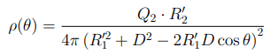
We have the density distribution, found in the previous sections of this article, given by the formula:

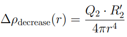
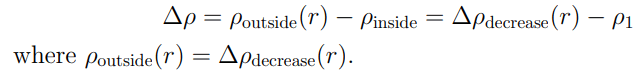
where r is the distance from the source to an arbitrary point, Q2 and R2′ are constants. We need to find the difference in density Δρ on the surface of the sphere.

Density difference inside and on the surface of the sphere

The density difference on the surface of a sphere of radius R1′ and inside it, as we defined when setting the problem, is given by the formula:

Formula for the space density distribution of the second charge on the surface of the first charge

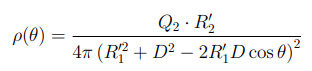
To calculate the gradient of the density on the surface of the first sphere (first charge), we first find the density’s dependence on the angle θ, using the formula for the distance on a sphere located at a distance D from the field source. The formula for the distance from the point to the source, obtained using the law of cosines, is well-known in geometry and does not require additional proof:

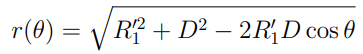
Now we substitute this expression for r(θ) into the formula for the density Δρdecrease(r):

Calculating the gradient of density on the surface of the first charge created by the second charge

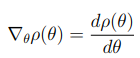
The density gradient on the surface of the sphere is defined as the derivative with respect to the angle θ:

dp(θ)/dθ

To calculate the density gradient with respect to the angle θ, we start with the expression for the density:

The gradient of density with respect to the angle θ will be equal to the derivative of this function with respect to θ:

Derivative of the density with respect to the angle

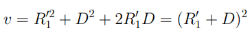
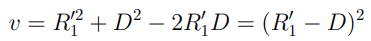
Let’s start by writing the derivative with respect to θ of the expression ρ(θ). We have a composite function of the form f (g(θ)), where g(θ)=R1′2 + D2−2R′1D cos θ.

Applying the chain rule, the derivative of the function ρ(θ) will be:

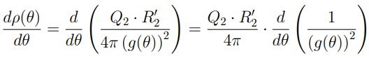
The derivative of 1/(g(θ))2 with respect to g(θ) will be:

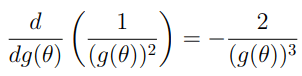
Now the derivative of g(θ) with respect to θ:

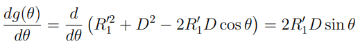
Finally, substituting these into the gradient:

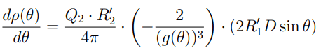
Simplifying, we get:

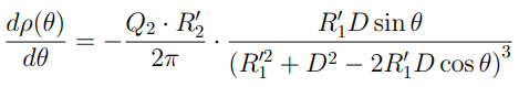
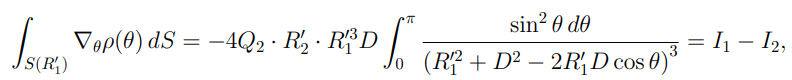
Now, we take the integral of this gradient over the entire surface of the first sphere to obtain the electric field acting on the first charge:

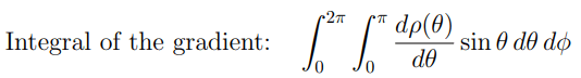
This integral gives us the total effect of the electric field, considering the perturbation of the space density distribution caused by the interaction of two charges [5,6]. The resulting formula will describe how the renormalization of charges and screening effects manifest when the distance between charges becomes comparable to their size, which is in agreement with QED predictions.

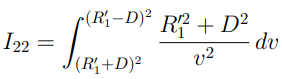
Consider each integral separately

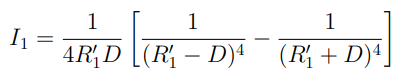
Solution of the first integral

Consider the first integral:

To solve it, we use the substitution:

The limits of integration will change as follows: When u=−1, v=(R1′−D)2. When u=1, v=(R1′+D)2.

Thus, the integral I/1 can be rewritten as:

This integral can be evaluated:

Substitute the limits of integration:

Solution of the second integral

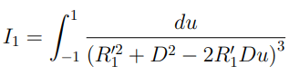
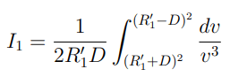
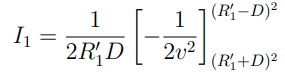
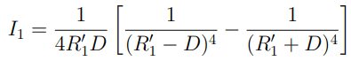
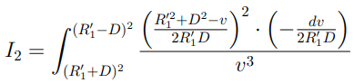
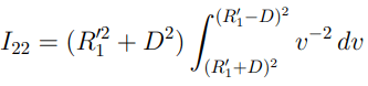
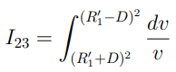
Consider the second integral:

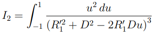
To simplify the integral, we first make a substitution. Use the substitution:

Then:

Now express u in terms of v:

Changing the limits of integration

When u=−1:

When u=1:

Thus, the limits of integration change from v = (R1′ +D)2 to v=(R1′-D)2.

Express the integral in terms of the new variable and substitute everything into the integral:

Factor out the constant multipliers:

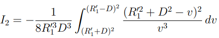
Now expand the square in the numerator:

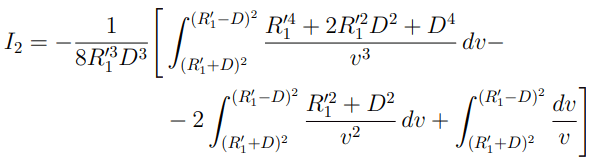
Decomposition into three integrals

Divide this integral into three separate integrals:

Now solve each of these integrals separately.

A.First integral:

Factor out the constants from the integral:

Evaluate the integral:

Substitute the limits:

B.Second integral:

Factor out the constants from the integral:

Evaluate the integral:

Substitute the limits:

C.Third Integral:

Evaluate the integral:

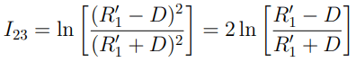
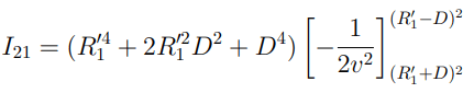
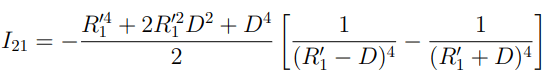
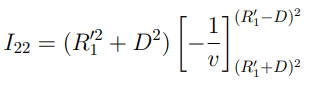
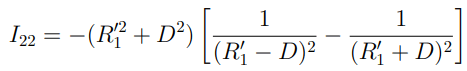
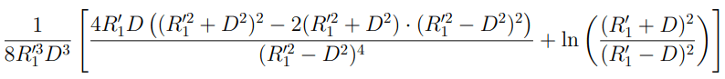
Substitute all three integrals into the expression and obtain the final expression for /2:

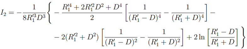
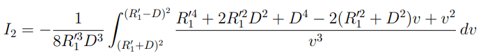
Now let’s simplify our expression for the integral I2, which is:

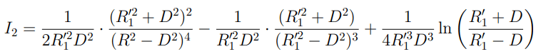
After simplification, we obtain the final expression for the integral of the gradient of the space charge density created by the second charge over the surface of the sphere of the first charge:

The solution for the first integral is:

The solution for the second integral is:

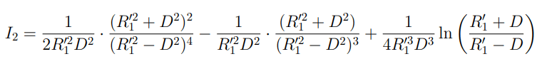
If we don’t factor out the exponent from the natural logarithm, we get the following expression:

Numerical investigation of the integral expression

We will investigate the obtained expression for the integral numerically. To ensure that the values of the integral do not enter the imaginary part, we will keep the expression for both the numerator and the denominator of the logarithmic term squared. The fact that for D

Here is an interesting result we obtained, which, in my opinion, fully corresponds to what was obtained at the quantum level for two charges at small distances within the framework of quantum electrodynamics (Figure 3).

FIG. 3. Graphs of the interaction quantity through the distortion of spherical symmetry of the field and through the direct interaction of the charge with the field of the second charge on the surface of the first charge’s sphere.

 

For comparison, here is how the electric field intensity graphs would look if we use the classical Coulomb’s law without correction for point charges, not considering their size and geometric shape (Figure 4).

FIG. 4. Graphs of the interaction quantity through coulomb’s law, with consideration for the interaction of the surface area of the first charge’s sphere with the field of the second charge.

 

We see that as the first charge approaches the field source, the field intensity starts to decrease, while the integral value of the gradient of the spatial density distribution over the surface of the first charge’s sphere begins to increase at distances on the order of 5 times the size of the first sphere. As the field source approaches the surface of the first sphere, the expression we obtained for the integral of the gradient over the surface of the first charge starts to decrease sharply, and this value quickly moves into the negative range [8-10]. At relatively small distances of the field source from the surface of the sphere, the value of the integral of the gradient over the surface of the sphere becomes greater in magnitude than the value for the amount of disturbance created by the second charge on the field of the first charge, meaning that at small distances the field starts to increase sharply, as predicted by Quantum Electrodynamics (QED) and confirmed by conducted experiments.

Thus, I have clearly shown that the proposed theory has a very wide range of applicability: It can correctly describe the behavior of the electromagnetic field at distances comparable to the size of the classical electron. The theory also correctly describes the interaction of charges as described by Coulomb’s law at large distances.

Using the formula, we obtained for the amount of energy required to compress a sphere creating an electric charge, which we interpreted as the mass of the charge, one can derive equations for the distribution of the curvature coefficient of the space metric and thus obtain the gravitational equations.

In my opinion, the theory I proposed and the approach used in it are the missing link that will connect processes, both gravitational and electro- magnetic, occurring at the quantum level with processes occurring at the macroscopic level. It can be said that the proposed theory is a statistical averaging of quantum mechanics at the macroscopic level, as it correctly accounts for the field effects associated with the sizes of the charges creating the field, the distribution of this field, and the interaction of charges both through direct interaction with the field and through the distortion of the field distribution created by each charge.

Conclusion

This work attempts to theoretically derive Coulomb’s law, which currently serves as an empirical generalized model of experimental data. The main goal of the study was to explain the fundamental interactions in nature by introducing a new concept space density which can quantitatively describe the distortion of space without changing its metric. This approach allowed us to propose a model that connects the concepts of gravity, electric fields, and the mass of matter on a deeper level than existing theories.

Main results

Derivation of coulomb’s law: Using simple mathematics and fundamental physical concepts, a formula analogous to Coulomb’s law was derived through the introduction of space density. This was achieved by recognizing that space density plays a key role in forming fields and forces analogous to those present in electromagnetism.

Concept of space density: Space density was introduced as a new physical quantity capable of describing space distortion. Unlike the traditional view of distortion through the metric tensor of space-time, this concept offers an alternative view of the interaction between matter and fields.

Space density was also linked to the concept of a “gravitational charge,” interpreted as the energy required to compress space. In this context, the gravitational charge explains how a “clump” of space density contributes to the distortion of the space metric and the creation of gravitational effects.

Further confirmation of the equivalence of energy and mass:

It is assumed that as the sphere S(R1) is compressed to S(R1′), where R1 is the uncompressed sphere with density ρ0, the gravitational charge corresponds to the amount of energy required to compress space. By integrating the force required to compress the space density from R1 to R1′ (whereR1>R1′), we obtained the energy required to compress the sphere, or the energy contained within the elementary particle, which determines the curvature coefficient of space along with its metric and forms what we currently understand as the mass of matter.

Our study once again confirms the assertion of the theory of relativity regarding the equivalence of mass and energy. This is important for understanding how energy is related to the curvature of space along with its metric.

Connection with existing theories

The paper shows that the proposed model does not contradict the laws of electrostatics, the theory of relativity, or quantum field theory but rather complements them, providing a deeper explanation of concepts such as matter, force, energy, and mass. In particular, the model confirms the existing views on the equivalence of the” creation energy” of elementary particles or their internal energy and their mass.

Comparison with existing theories

The introduction of space density as a mechanism responsible for distortion provides a way to integrate it with established theories such as general relativity and quantum field theory. Space density can be associated with the gravitational charge, which causes the distortion of the space metric tensor, aligning with ideas about the Higgs boson and its role in endowing matter with mass.

Philosophical aspects of physics

The work touches not only on the technical aspects of deriving physical laws but also on philosophical questions about the nature of matter and energy. This makes the theory a universal platform for further research in fundamental physics.

Final remarks

The concept of space density proposed in this work represents the first but very important step toward creating a unified theory of everything, which unites gravitational and electromagnetic interactions and explains the nature of mass in matter. The derivation of a formula analogous to Coulomb’s law and the understanding of mass as the amount of energy required to compress space provide a new and very interesting foundation for studying physical processes.

However, many questions remain open. At present, space density remains a hypothetical quantity, and the mechanisms that cause its specific behavior require further study. Future research should focus on experimentally con- firming the proposed ideas and on a deeper theoretical understanding of the mechanism of interaction between space density, matter, and fields.

Thus, this work is the first step toward a more profound and comprehensive theory that requires collective efforts and further development. This new approach has the potential to lead to fundamental discoveries and revolutionize our understanding of the nature of forces, fields, and matter.

References

1. Dyson FJ. The S matrix in quantum electrodynamics. Phys Rev. 1949;75(11):1736.

   [Crossref] [Google Scholar]

2. Feynman RP, Leighton RB, Sands M, et al. The feynman lectures on physics; vol. i. Am J Phys. 1965;33(9):750-752.

   [Crossref] [Google Scholar]

3. Kaluza T. On the Unification Problem in Physics, Sits. Press Akad Wiss Math Phys K. 1921;1:895.

   [Crossref] [Google Scholar]

4. Klein O. Quantentheorie und fünfdimensionale Relativitätstheorie. Zeitschrift für Physik. 1926;37(12):895-906.

   [Crossref] [Google Scholar]

5. Appelquist T, Chodos A, and Freund PGO. Kaluza-Klein Theories, Addison-Wesley, 1987.
6. Appelquist T, Chodos A, Freund PG. Modern Kaluza-Klein Theories. 1987.

   [Google Scholar]

7. Feynman RP. Quantum Electrodynamics WA Benjamin. Inc. NY. 1961.
8. Feynman RP. Feynman lectures on physics. Volume 3: Quantum mechancis. Reading. 1965.
9. Feynman RP. QED: The Strange Theory of Light and Matter Princeton University Press. Princeton, New Jersey. 1985:p15.
10. Feynman RP. Space-time approach to quantum electrodynamics. InQuantum Electrodynamics 2018 Feb 19 (pp. 178-198). CRC Press.