Original Article
, Volume: 6( 1)Probability, Randomness, and Subspace, with Experiments
- *Correspondence:
- Solomon BT , Chairman, Xodus One Foundation, 815 N Sherman St., Denver, CO 80203, USA, Tel: 310- 666-3553; E-mail: bts@XodusOneFoundation.org
Received: December 06, 2016; Accepted: January 06, 2017; Published: January16, 2017
Citation: Solomon BT, Beckwith AW. Probability, Randomness, and Subspace, with Experiments. J Space Explor. 2017;6(1):110.
Abstract
Quantum theory does not have a mechanism that explains how nature implements probabilities. Thus, the main objective of this paper is to present new directions in the understanding of probabilities and randomness with the eventual objective of controlling photon localization (in a future paper). The expectation is to improve photon collection and loss mitigation. The conservation of energy within the photon’s transverse electromagnetic wave requires that energy is transferred between spacetime (x,y,z,t) and subspace (x,y,z). This paper proposes that it is in this subspace that nature implements probabilities. The paper analyses the differences between probabilities and randomness and infers that all particles have internal clocks C, that is the mechanism for randomness. A glass thought experiment is used to clarify how probabilities are effected and as a result it is proposed that the random distribution of photons across the Point Spread Function or Airy Pattern (not Airy Disc) is not due to the photon probability but due to the random behaviour of electron shells receiving the photon localization. Finally, 5 experiments are proposed.
Keywords
Photon localization; Photon probability; Born’s interpretation; de Broglie; Airy Pattern; Photon propagation; Randomness; Probability; Schrödinger wave function; Bell’s theorem probability
Introduction
One of the objectives of this paper is to provide an alternative model to the fundamentals of physics, the precursor or prerequisite to quantum theory. It is not about building a better quantum theory. That is unlikely given that over the last 100 years, thousands of expert physicists have checked, double and triple checked this theory as it stands. With an alternative to the foundations of physics one can then falsify (technical usage) quantum theory with three possible outcomes. (i) The foundations of quantum theory are correct and alternative fundamentals are incorrect, resulting in a strong better quantum theory, (ii) The proposed foundations of physics lead to a different and better version of quantum theory or (iii) The interplay between both version, contemporary and proposed foundations, lead to more questions than answers.
Quantum theory describes both mass-based particles and massless particles as exhibiting wave-particle duality. Experimental confirmation of this duality can be found [1] such that
• The photon particle behaviour can be demonstrated by the photoelectric effect (given a work function W) of energy E with frequency ν as,
E = hν -W (1)
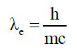
• The electron’s wave behaviour can be described by Compton’s scattering. A photon scattered at angle θ has a longer wavelength λ1 given the electron’s Compton wavelength λe, and
λ1- λ= λ1 (1-cosθ) (2)
 (3)
(3)
• The de Broglie’s matter wave, that mass matter and massless light satisfy the same energy-momentum and momentum-wavelength (p-λ) relationship,
 (4)
(4)
Quantum theory’s wave mechanics is described by the Schrödinger wave equation Ψ (x,t) per
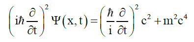 (5)
(5)
Giving Born’s interpretation of |Ψ|2 as the probability density of finding system at space time location (x, t),
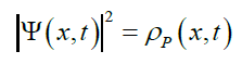 (6)
(6)
Such that the probability density can be moved around, but cannot be created or destroyed in the absence of explicit creative or destructive physical processes. As the physical states in quantum mechanics are linear waves they can be superposed to form other waves using Fourier transforms. And a wave of any kind satisfies the uncertainty relation that for matter waves is the Heisenberg uncertainty principle
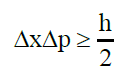 (7)
(7)
Therefore, one notes that quantum theory is essentially a wave theory used to describe particle behaviour, with all non-wave properties (probabilities for example) described in terms of this wave nature. Photons in particular are also modelled using wave equations known as Bessel functions. As Roychoudhuri [2] proposed, “We need to embark anew on comprehensive foundational studies about generation, propagation, and detection of EM waves across the entire spectrum. Huygens- Fresnel’s wave picture and Einstein-Dirac’s indivisible quanta represent one of the strongest unresolved issues in physics.”
While the authors agree with his premise for the need for foundational studies, Roychoudhuri [2] has undertaken these foundational studies using wave equations. In this paper the authors take a different approach, by laying the ground work required to model photon behaviour in terms of probabilities instead of wave equations or Bessel functions. How is this possible?
In Operations Research, there is a class of mathematic search techniques, mathematical programming, that have a unique property known as primal-dual formulation. Mathematical programming consists of an objective function that is matrix row, a matrix of constraints whose inequalities form a matrix column of boundary conditions, known as the Primal problem. The dual problem occurs when the constraint matrix rows and columns are swapped, and concurrently, the objective function is swapped with the boundary conditions. It turns out that the solution to the Primal formulation is identical to the solution of the Dual formulation. That is, two apparently different formulations of the same problem have identical solutions.
The point spread function (PSF), here termed Airy Pattern (not Airy Disc), of photons projected through a pin hole to a screen, is the basis of this deconstruction. However, the modern definition of this type of PSF is a Bessel function expressed only in terms of wave functions and therefore not suitable for the proposed deconstruction, as the Bessel functions have entirely removed the photon’s probabilistic behaviour. The wave Bessel functions can be considered the primal formulation. To determine the probabilistic behaviour, the dual formulation, one must go back to the older formulation (Appendix A and B) of the Airy Pattern. As proof that this dual formulation exists, the probabilistic dual formulation should give identical results to the Primal Bessel formulation. This will be shown correct in a later paper (Figure. A1).
Roychoudhuri [2] summarizes that there are two types of photon models, (a) Huygens-Fresnel’s wave and (b) the Einstein-Dirac’s indivisible quanta. As Roychoudhuri [2] states, the definition of a photon by quantum electrodynamics is something like an indivisible packet of energy but represented by a Fourier monochromatic mode of the vacuum which is problematic, for the following reasons
(i) Such individual photons cannot be localized in space and time.
(ii) An infinitely long Fourier mode violates the principle of conservation of energy
(iii) Superposition of many Fourier frequencies creating a space-finite pulse in free-space to model pulsed light is an invalid conjecture because waves cannot interact and regroup their energies in the absence of interacting materials.
(iv) It assigns rich properties to “vacuum” and yet relativity and quantum physics do not explicitly recognize space as a physical medium.
(v) The quantum photon’s indivisibility directly contradicts the immensely successful HF diffraction theory.
Solomon [3] pointed to the need for a more sophisticated space time. Using Roychoudhuri’s critique as a basis for comparison, one can state that this paper lays the ground work for a third model derived from the Airy Pattern, an infinitely thin disc whose plane (x-y axes) is orthogonal to the photon’s motion vector along the z-axis, that is not infinite (per ii), and based on a “richer” (per iv) property of space time, one that involves both deformable space time (x, y, z, t) and deformable subspace (x, y, z).
Further, there is in physics research, what is known as the pilot model [4], which has a specific re-interpretation of probability, and not just on the basis of wave interference. “The Copenhagen interpretation is essentially the assertion that in the quantum realm, there is no description deeper than the statistical one. When a measurement is made on a quantum particle, and the wave form collapses, the determinate state that the particle assumes is totally random. According to the Copenhagen interpretation, the statistics don’t just describe the reality; they are the reality. “ [5]
The research in this paper is to determine another layer of statistical inference, as an alternative to the Copenhagen interpretation, and that is what the offered aim of this paper is.
Definition of Kenos
This paper proposes that photon localization is not due to the wave function collapse per quantum theory is a result of• the αβ join between the α space time and the β subspace. To do this it is necessary to deconstruct the photon’s wave function ψP into its probability density function φP and remaining components.
Is there evidence for both the spacetime α kenos and subspace β kenos? Yes, it is found in the conservation of energy within• a photon. See Appendix A and B for discussion on a proposed particle structure.
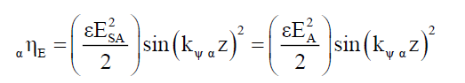
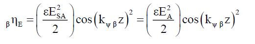
For a, given photon wavelength λ the electric ηE and magnetic ηM field energy densities along the z-axis are given by,
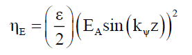 (8)
(8)
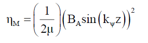 (9)
(9)
Where EA and BA are the maximum amplitudes of the electric and magnetic fields respectively in spacetime, and kψ is the wave function constant,
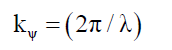 (10)
(10)
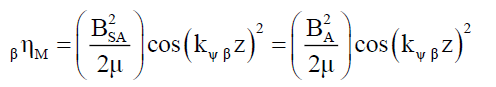
As the transverse wave’s electric EA and magnetic BA field oscillates in unison, the energy densities (8) and (9) oscillate between 0 and maximum (or 100%), thus breaking conservation of energy at any specific point in the transverse wave in spacetime.
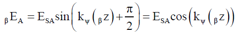
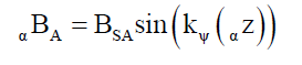
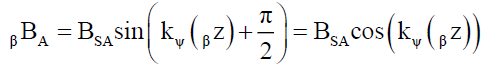
One approach to solving this oscillating energy is to propose that the electromagnetic transverse wave’s electric EA and magnetic BA vectors are the projections of the electric ESA and magnetic BSA super vectors rotating orthogonally about their axis of motion, between the spacetime α kenos and the subspace β kenos.
This is equivalent to a rotating clock hand in the x-y plane moving along the z-axis, with the projection of this clock hand on the y-z plane is 90° out of phase with that in the x-z plane. Thus, these α and β kenos projections of the electromagnetic wave are 90° out of phase.
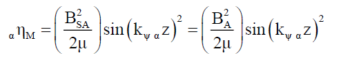
Then the strengths of their respective electric αESA and βESA and magnetic αBSA and βBSA field projections in their respective α kenos and β kenos are given by,
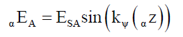 (11)
(11)
 (12)
(12)
 (13)
(13)
 (14)
(14)
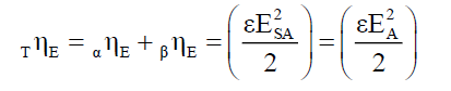
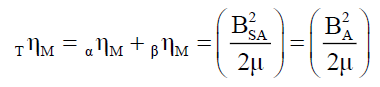
This paper proposes that the energy in space time is the same as energy in subspace. The total electrical energy density TηE and total magnetic energy density TηM are the sum of their respective electrical αηE and βηE and magnetic αηM and βηM energy density components in the space time kenos α and subspace kenos β, respectively, such that these total energy densities are always constant,
 (15)
(15)
Where,
 (16)
(16)
 (17)
(17)
And,
 (18)
(18)
Where,
 (19)
(19)
 (20)
(20)
Thus, both the total electric TηE and total magnetic TηM field energy densities are constant at any given point along the transverse wave displacement. Note that, the electromagnetic energy Eem is not a function of the field strength of these field vectors per (21). It is purely a function of the field super vectors’ rotation about the axis of motion which one observes as a frequency projection ν in spacetime.
 (21)
(21)
That is, as the super vectors rotate, the amplitudes of these field vector projections oscillate, within their respective spacetime α kenos and subspace β kenos. Thus, so do their field energy densities in their respective kenoses. Therefore, a strict treatment of conservation of field energy within the photon proves that both the spacetime α kenos and subspace β kenos exists. Equally important, one notes field energy conservation holds because energy can be transferred between kenoses.
The question that quantum theory does not ask is, how does Nature implement probabilities? Photon localization events are space but not time dependent as probability fields are time invariant. Therefore, the probability field is a region of space or kenos where time does not exist thus Solomon [7] proposed that nature implements probabilities in the subspace β kenos and not in the spacetime α kenos. And therefore, for a localization event to occur between the subspace β kenos probability field• and the spacetime α kenos localization, a join must occur between subspace β kenos and space time α kenos at that location.
Of course, much work remains to done as to the properties of subspace and these super vectors. This, however, raises another question, energy in spacetime is usually associated with motion as in kinetic energy, how then is field energy expressed in subspace that does not have the time dimension? One possibility is potential energy. Since the only two observable properties are electric and magnetic field energies and probabilities that are 90° out of phase, one could infer that this potential energy takes the form of a probability structure in subspace, just as gravitational energy is observed as a structure of space time. Thus, equating electric field energy (electric field energy density αηE x volume VE occupied by this electric field) (15) to probability density PψP, from C5 and B8 in Appendix C and B, respectively,
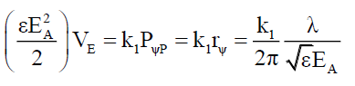 (22)
(22)
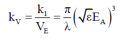 (23)
(23)
Where k1 and kV are some coefficients. Further work will be published in a future paper as this research is still in its infancy. This paper proposes new directions in investigating how probabilities are implemented in Nature.
A definition for localization and randomness
To extricate additional probabilistic relationships a Glass Thought Experiment (GTE) was proposed [5,6]. Figure. 1 illustrates this GTE. Photons having passed through the transparent screen form Airy Patterns on the opaque screen with their respective envelope probability density function φA,T and φA,O. This GTE illustrates several properties
(i) ΦA, O ≠ 0: Figure. 1a shows that for any distance between pinhole and screen, moving the opaque screen back and forth demonstrates that the photon probabilistic envelope probability density function φA exists in the space between the pinhole and opaque screen.

Figure 1a: Opaque and transparent screen Airy Patterns.
(ii) φA,T ≡ φA,O: Figure. 1(a) shows that the PSF Airy Pattern on the opaque screen demonstrates that the photon’s probability distribution is intact after having passed through the transparent screen.
(iii) hν: In the transparent screen, the Airy Pattern are not discernible as the electromagnetic function does not interact with the screen. In the opaque screen, the electromagnetic function does interact with the screen to form• the PSF Airy Pattern. That is the electromagnetic energy hν and therefore frequency ν is a necessary criterion for• interaction.
(iv) Ai ≠ f(Pi): the electromagnetic function’s ability to interact Ai with the material is independent of the photons envelop probability function or its probability to interact Pi. This is because the photon interacts (Ai=1) with the opaque but not (Ai=0) with the transparent visual plane even if the two planes are attached together, φA,T=φA,O or when they are far apart, φA,T ≠ φA,O.
(v) Pi = f(φP) ≠ f(Ai): On both screens the probability to interact Pi is determined by the envelop probability density function and not by the material. This is because the probability to interact Pi is independent of the opaque screen and is present even when no interaction is observed. Ignoring edge diffraction effects to keep it simple, Figure. 1b shows that an opaque barrier can effectively neutralize the photon probability distribution in that region where the barrier exists.

Figure 1b: Blocked photon probabilities.
(vi) ∫ Pi dx=1, in a confined space the φA distribution along all and any radii x must total 1.
By iii) given that the photon frequency is the appropriate frequency, one notes that by iv) the ability to interact Ai=1 is independent of the probability to interact Pi by v). This raises an interesting inference. Probabilities exists in nature but to effect photon localization a trigger is required. Since photons only localize on the electron shell, given iii), a unique and individual atom’s electron shell experiences a trigger event such that for any given identical set of atoms in the local vicinity, the one with this trigger event will receive the photon while the others are not ready to do so. The proof of this trigger event can be seen as individual specs that form the Airy Pattern. There are billions of atoms in the opaque screen that are capable of receiving the photon, but only one receives it at any one time, not the others.
What is this trigger? It is proposed that it is the αβ join between spacetime α kenos and subspace β kenos. When this αβ join occurs in the electron shell, the electron shell is able to interact with the photon’s envelope probability density function φA and is captured by this electron shell. That is, in the presence of the photon’s probability density function φA, localization is the process of the photon capture due to the formation of an αβ join between spacetime α kenos and subspace β kenos in the electron shell.
Therefore, two inferences are in order. First, in a dynamic electron shell, spacetime α kenos and subspace β kenos, αβ joins are continuously created (open or Ai=1) and destroyed (closed or Ai=0). Second, the spatial randomness of the photon specs on the PSF Airy Pattern is the result of the uniform distribution of electron shells that observe a temporal randomness of the opening and closing of these joins by individual electron shells. That is, the act of randomness is not the effect of the photon’s probability density function φP, but of how a collective of electron shells respond to photon arrivals. Which raises the question, is it possible to accelerate αβ joins in a specific region of the opaque screen as to demonstrate a spot within the PSF Airy Pattern?
Therefore, as Nature has demonstrated the spacetime-subspace αβ joins, these αβ joins are technologically feasible. However, experiments are required to describe how to influence these αβ joins.
A theoretical formulation for randomness and probability
Khrennikov [8] has stated “Bell's theorem rejects only local hidden variable models, i.e. models preventing faster than light communications.” Bell’s theorem is limited to spacetime. However, as shown in this paper, the conservation of energy within the electromagnetic transverse wave requires both the existence of the spacetime and subspace. In this light Bell’s theorem is inapplicable.
Much of the discussion in the section is either borrowed from, extends, or modifies the discussion presented by Khrennikov [8].
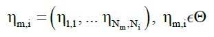
Axiom 1, States η: Fundamental states η (for example particle spin) must have Nη unique values,
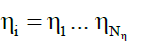 (24)
(24)
And not be correlated or associated i.e. they are independent of each other. If any two states, for example η1 and η2 are not independent then at least one of them is a pseudo-state. They may both be dependent on a third state η3, and in general,
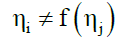 for i≠j (25)
From the perspective of randomness,
i>1
As when i=0 no states exist, and when i=1 the state does not change.
Axiom 2, Receptacle ρ: A receptacle ρ is a fundamental carrier of the states ηi,
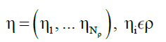 (27)
(27)
Axiom 3, collection Σ: A collection Σ (for example a fundamental particle) is a collection of Nρ receptacles ρi,
 (28)
(28)
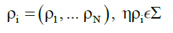
Axiom 4, true independence: True independence occurs when, within the same collection Σm, any state j of receptacle i or state l of another receptacle k is independent of each other,
 for i≠k and j≠l (29)
Axiom 5, sequence Θ: A sequence Θ is a set of states that are associated in space or time. Necessarily, by the earlier discussion, this sequence of each state i must belong to different collections Σm.
 (30)
(30)
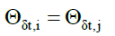
Axiom 6, spatial randomness: In addition to (25) and (29), given a local space δl,
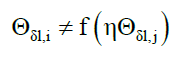 for i≠j (31)
Even though,
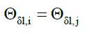 for i≠j (32)
For example, spatial randomness is the localization of a photon i at electron shell i and is independent of the localization of photon j at electron shell j, separated by a local spatial distance δl, even if both photon-electron-shell localizations are identical processes. This can be extended to multiple sets of photo-electron-shell interactions.
Axiom 7, temporal randomness: In addition to (25) and (29), given a local time difference δt,
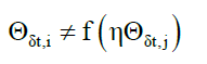 for i≠j (33)
Even though,
 for i≠j (34)
For example, temporal randomness is the localization of a photon i at electron shell i and is independent of the localization of photon j at electron shell j, separated by a local spatial time δt, even if both photon-electron-shell localizations are identical processes. This can be extended to multiple sets of photo-electron-shell interactions.
These axioms 1 to 6, necessarily imply that the change in the value of a state η is independent of the world outside the receptacle ρ and is only a function of time tc or the receptacle’s internal clock C,
 (35)
(35)
Obviously, in a flat spacetime, these internal clocks C do not change with spatial distances or else the laws of physics would not be the same everywhere. That is, von Neumann’s principle of sufficient cause [4] does not operate at the level of states.
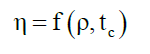
Therefore, one infers that randomness originates from fundamental particle internal clocks C. A generic definition of a clock is a stable and precise repeating process or a mechanism. Examples are rotation and simple harmonic motion. Therefore, frequency would be a suitable candidate for an internal clock. This suggests that photons do not have a process (38) of converting internal clocks to random states η. i.e. photons on their own, are not capable of generating random states. This is because, in the absence of particle based external structures, photons are observed to be very stable. Examples include atomic spectral lines from any star from any galaxy in the Universe. This stability points to the lack of the process (38) of converting internal clocks to random states η. One infers unlike Khrennikov [8] that probabilities and randomness are different phenomena.
Per Axiom 6 (31) and (32), the Airy Pattern B1, Appendix B, screen can be defined as a 2-dimensional spatial sequence ΘA, which causes the randomness. The relevant states ηJ=(0,1) are the αβ spacetime-subspace joins closed/inactive or open/active, respectively. Some inferences come to mind.
• In this Airy Pattern sequence ΘA, the number ηJ0 of closed states is much greater than the number nJ1 of open states, otherwise rAU would not be very, very large as photons would be captured “quickly”.
• These join states ηJ are truly random else they would alter the Airy Pattern probability distribution, and different screen materials would evidence different Airy Patterns (Table B1).
Since, localization occurs when ηJ=1, the Airy Pattern localization event LA can be written as a series of recursive transformations in terms of the photon probability PP and transformations ∇n at each step n that transforms this probability,
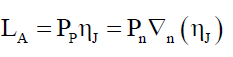 (36)
(36)
The recursive transformations ∇n where n>0 is such that,
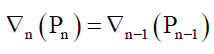 (37)
(37)
With n=0 is the state ηJ. Or,
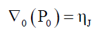 (38)
(38)
P0 is the process that converts this internal clock to Join states of η=0 or η=1, and ∇0 (=∇ψ,J) is the transformation that converts the Join states into probability functions that can interact with the external probability field. Unlike the recursive function presented in Khrennikov [8] which leads to complexity, the finite (n is small approximately n ≤ 8) recursive function (37) unravels by decreasing n. That is, n is not a very large number and this limits the complexity observable in nature. Therefore, the random nature of states η due to the internal clocks C, are the source of randomness. That is, von Neumann’s principle of sufficient cause [8] only operates for n>0. It also means that the Copenhagen interpretation “there is no description deeper than the statistical one” is no longer valid.
Therefore, one can infer some necessary conditions.
• n=0: P0 converts the state η into a form that ∇0 can be transformed into a wave function form.
• n=1: This is the transformation of the distorted photon’s wave function’s ψA interaction, the Airy Pattern on the opaque screen, with the states η to probabilities, i.e. the first contact with the random event P0(∇0)=ηJ.
• n>1: transformation of the various probability densities into other probability densities.
• Last n: transformation of the last probability density into the final photon wave function ψP.
• Probability Density: Ville’s Principle states that “a random sequence should satisfy all properties of probability one.” Thus, given a probability density function ψP along a radius rP,
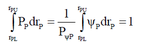 (39)
(39)
as PψP (=4/π, see Appendix C) is a pre-calculated known constant. Therefore, given a density Dr, (39) can be rewritten as,
 (40)
(40)
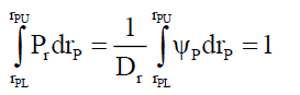
For example, the point probability along a radius rP must sum 1. The probability Pθ of any radius must also sum to 1, and is• given by,
 (41)
(41)
That there is recursion,
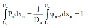 (42)
(42)
Where Ln and Un are the lower and upper limits of the integrals at stage n and xn is the variable integrated. (42) is equivalent• to (37). That is, Ville’s Principle is correct under strict conditions that each stage n is derived from the previous n-1 stage, but probability PP is not the source of internal clock’s C randomness and therefore C by itself, does not obey Ville’s Principle. From a particle structure perspective, one notes that all particles must have, as a part of their construction, internal clocks C. That is, it is the wave function in contact with an open join at an electron shell interacts with it. These open joins are caused by the randomness of electron shell states. Probability distributions on the other hand, spread the possibility of this interaction• over a spatial region. This spread is determined by the presence or absence of other transformations ∇i in its vicinity.
Propagation versus probability
If the photon is directed at the PSF Airy Pattern opaque screen its arrival time tA should be the distance dA between pinhole and opaque screen, divided by the velocity of light c.
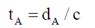 (43)
(43)
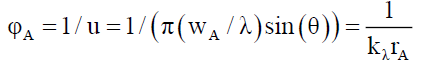
The Solomon [7] proposed that the basic particle structure is an infinitely thin wave function disc C1 (Appendix C), that is orthogonal to the particle’s motion vector (like a flat umbrella with other particle properties added to this structure). In terms of the space wave χP, the envelope probability density function φP this ψP wave function when projected [7] on to the opaque screen forms the Airy Pattern ψA (44) and its corresponding space wave χA (45), and envelope probability density function φP (46), given the pinhole aperture diameter wA, the distance between pin hole and screen dA and angular displacement θ from pinhole a radial position rA on the screen,
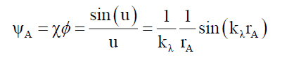 (44)
(44)
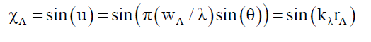 (45)
(45)
 (46)
(46)
Where, for small θ,
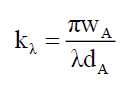 (47)
(47)
That is, there is a transformation of the particle’s ψP wave function C1 Appendix C, to the Airy Pattern ψA pattern (44). See• Figure. 2.

Figure 2: Probabilistic wave solution ψ (solid red) and its 2 components, χ (dashed grey) and φ (dot-dash green).
As this projected wave function (44) travels the distance dA this paper proposes that all photon arrivals are equal and requires a time of tA to arrive at the opaque disc. The path from pin hole to an orthogonal displacement at the opaque screen can be divided into two parts. First, the propagation from pinhole to opaque screen, and second, translocation, the orthogonal probabilistic localization in zero time at a radial displacement from pinhole axis. The experimental proof would be to prove that all photon arrival times (43) are only dependent of the distance between pinhole and opaque screen, and independent of• the hypotenuse travel path i.e. independent of their localization distance along the radius from the axis of propagation.
Proposed experimental tests
This paper proposes four new experiments that photonics researchers can conduct to confirm or disprove the probability control hypothesis presented in this paper.
Test for subspace
As noted in section 2, the electromagnetic vector rotates between spacetime and subspace, and these are out of phase by 90°. Therefore, it should be possible to demonstrate that the electric field induced voltage is out of phase with photon localization• by 90° as depicted in Figure. 3.

Figure 3: Proposed experiment depicting voltage and localization out of phase by 90°.
Test for probability versus propagation
If the envelope probability and the space wave are the cause of the interference and diffraction patterns, then one would expect, as depicted in Figure. 4, that the hypotenuse travel time th and the direct travel time td, should be equal,
 (48)
(48)

Figure 4: Proposed experiment for propagation versus probability.
The inference is that the electromagnetic function and the combined envelope probability and the space wave are primal-dual. In operations research’s, primal-dual solutions are identical where the primal problem is defined by an objective (row) function, a constraint matrix and column of limiting values of each constraint in the matrix. The dual problem exists when the columns and rows are swapped.
Test for probability versus randomness
If probability and randomness are two separate phenomena, with randomness due to the material, then it is in theory possible to modify the randomness of selected parts of the PSF Airy Pattern, and demonstrate (i) a bright spot on the PSF Airy Pattern with decreased localization in the remaining PSF Airy Pattern, and (ii) a dark spot on the PSF Airy Pattern with increased localization in the remaining PSF Airy Pattern. See Figure. 5a and Figure. 5b respectively. The bright spot would be caused by materials whose join occurs more frequently than the opaque screen, and vice versa, the dark spot caused by a material whose join occurs less frequently than the opaque screen [9].

Figure 5a: Bright spot proposed experiment.

Figure 5b: Dark spot proposed experiment.
A test for the mechanism behind quantum entanglement
Locality demands the conservation of causality, meaning that information cannot be exchanged between two space-like separated parties or actions [10]. Quantum entanglement can be described [11] as non-local interactions or the idea that distant particles do interact without hidden variables.
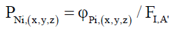
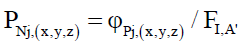
There are two possible alternative explanations that do not require hidden variables. First, that subspace is the carrier of this entangled information, and second is the envelope function φP based spatial probability distribution. Note, since photons do not exhibit randomness, the process (38) of converting the internal clock to Join states of η=0 or η=1, are not present and therefore, entanglement cannot be due to internal clocks C. The spatial probability distribution is so large, that entanglement occurs while the entangled photons’ probability fields overlap. The joint probability Pij,(x,y,z) (49) at coordinates (x, y, z) of photon i interacting with its entangled photon j is the product of the individual probabilities Pi,(x,y,z) and Pj,(x,y,z).
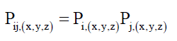 (49)
(49)
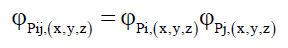
Given that these particle probabilities obey the envelope function φP C3, (49) can be written as (50),
 (50)
(50)
The normalized probabilities PN would take the form,
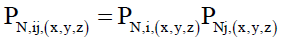 (51)
(51)
with,
 (52)
(52)
 (53)
(53)
Assuming that the particle must arrive at the detector, the denominator is the field of interaction FI,A’. This is the area FI,A’ of the curved surface of the detectors used in the experiments. This denominator can be simplified to FI,A by only considering photon arrivals through the cross section of the detector aperture as opposed to detector surface.
If entanglement is due to the joint probabilities of the envelope function φP then two scenarios can be formulated
• Two un-entangled independent photons i and j with their envelope terms φPi and φPj pass through their respective double slits, will exhibit the normal interference patterns. Mathematically, by linear superposition, these are the straight sum ΣnψPn of their respective, probabilistic wave solution ψPn, for n=i and j, and A5 would hold, such that (Figure 6),
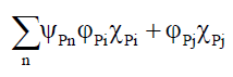 (54)
(54)

Figure 6: Airy Pattern interference of 2 entangled photons with independent envelop probabilities.
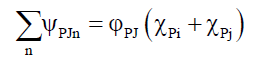
• If two entangled photons i and j exhibit joint probabilities, then their envelope terms φPi and φPj are replaced by their joint probability envelop term φPJ, (55), such that the joint probabilistic wave solution ψPJn by linear superposition and A5, would take the form (Figure 7).
 (55)
(55)

Figure 7: Airy Pattern interference of 2 entangled photons with joint envelope.
For ease of illustration, Figure 6 and 7, the photons i and j are separated by 1m with the probabilistic wave functions mapped out on a 10m square screen, positioned 1m away from their apertures.
It is clear that the resulting interference patterns are different and therefore a test of the validity of subspace versus joint probability. If subspace is the carrier of entangled information one should observe interference patterns similar to Figure 6, else if joint probabilities are the carrier than one should observe interference patterns similar to Figure 7.
Conclusion
To understand the fundamentals of particle behavior, this paper has proposed that (i) all particles have internal clocks, (ii) and some particles can convert this internal clock into random states necessary for photon localization. The particle wave equations and probabilistic behavior are primal-dual problem formulations. Therefore, this paper proposes that probabilities and randomness are two different phenomena that can be traced back to particle properties. Finally, the paper proposes several experiments to test the thesis that probabilities are implemented in subspace, and a test for how entanglement could be implemented in Nature.
References
- Wong CW. A review of quantum mechanics, review notes prepared for students of an undergraduate course in quantum mechanics. Department of physics and astronomy, University of California, Los Angeles, CA2006;2016.
- Roychoudhuri C. Causal physics: Photons by non-interactions of waves, CRC Press, Boca Raton; 2014.
- Solomon BT. New evidence, conditions, instruementsandexperiments for gravitational theories.J Mod Phys. 2013;4:183-96.
- Bohm D. A suggested interpretation of the quantum theory in terms of hidden variables, II". Phys Rev. 1952;85(2):180-93.
- http://news.mit.edu/2014/fluid-systems-quantum-mechanics-0912
- Solomon BT. Non-Gaussian photon probability distributions, in the proceedings of the space, propulsion and energy sciences international forum (SPESIF-10). Robertson GA, editor. AIP conference proceedings 1208, Melville, New York; 2010.
- Solomon BT. Super physics for super technologies: Replacing Bohr, Heisenberg, Schrödinger and Einstein. Propulsion Physics Inc. Denver; 2015.
- Khrennikov A. Randomness: Quantum versus classical. Quantum Physics; 2015.
- Solomon BT, Beckwith AW. Photon probability control with experiments. Physics Essays; 2016.
- Eisaman MD, Goldschmidt EA, Chen J, et al. Experimental test of nonlocal realism using a fiber-based source of polarization-entangled photon pairs. Phys Rev. 2008;77:032339p.
- Howell JC, Bennink RS, Bentley SJ, et al. Realization of the Einstein-Podolsky-Rosen paradox using momentum and position-entangled photons from spontaneous parametric down conversion. Phys Rev Lett. 2004;92(21):1-4.