Research
, Volume: 0( 0)The study of GPS TEC and its comparison with IRI-2016 and NeQuick2 predictions at Sonmiani during high solar activity period of solar cycle 24
- *Correspondence:
- Muhammad Atiq , PhD Student in Institute of Space and Planetary Astrophysics (ISPA), University of Karachi, Karachi - 75270, Pakistan, Tel: 99261300-07; Fax: 99261340; E-Mail: muhammadatiq80@gmail.com
Received: July 16, 2018; Accepted: August 02, 2018; Published: August 07, 2018
Citation: Atiq M, Ameen MA, Sadiq N. The Study of GPS TEC and its Comparison with IRI-2016 and NeQuick2 Predictions at Sonmiani during High Solar Activity Period of Solar Cycle 24. J Space Explor. 2018;7(3):147
Abstract
The temporal variations in Total Electron Content (TEC) calculated from GPS (Global Positioning System) signal has been analysed at low latitude station Sonmiani (25.19° N, 66.75° E) during the high solar activity (HSA) period from May 2014 to September 2015 of the most recent solar cycle (SC) 24. It has been found that the diurnal variations in GPS TEC show peak value around post noon hour, 1500 LT (local time). The GPS TEC shows high values in equinoctial months as compared to solstice months. The winter anomaly is present in daytime with relatively large amplitude in the year 2014 as compared to 2015. It is completely absent during nighttime. It has been found that IRI-2016 model TEC shows both positive and negative deviation. The model underestimates the GPS TEC most of the time. The critical frequency of the F2 layer (foF2) obtained from NeQuick model by ingesting GPS TEC has been compared with IRI – 2016 foF2 and good agreement is found around June solstice and December solstice. The root mean square error (RMSE) in GPS TEC has been found large in equinoctial months. In iterations process at Sonmiani that the 70% points gives tolerance of ±1 MHz and the 17% of the total iteration showed ΔfoF2 = 0.
Keywords
TEC, IRI, CV, GPS, foF2
Introduction
The Global Positioning Satellites (GPS) is an arrangement of satellites propelled at the 20,200 km (approx.) height for correspondence reason. This program was begun in 1960's and afterward satellites are launched well ordered to build the coverage area on the Earth's surface. The signals from the GPS satellites go through the ionosphere during directly affect the GPS signal. The two kinds of impacts of ionosphere on the GPS signal are phase advance and group delay. In GPS signal the carrier signal is of much high frequency as comparable to modulating signal and these results into a change in speed when these signal passes through the ionosphere. As we know that the refractive index depends upon the wavelength of signal, therefore changing speed is associating with the change in wavelength and hence two signals phase and group contain different refractive indices when passing through the ionosphere. The refractive index for phase speed is less than 1 while for group speed it is greater than 1. For vacuum it is equal to 1 for electromagnetic signal. This produces time delay in modulating signal [1-5].
The ionosphere in the equatorial and low latitude region shows some anomalous features in diurnal, seasonal and annual variations. These anomalous features are called “Anomalies”. The most prominent is the Equatorial Ionization Anomaly (EIA) region with ± 30° of magnetic equator. In EIA region the electron density variations shows maximum at ± 30° of the magnetic equator and minimum at magnetic equator. The EIA region of the ionosphere has been the most challenging and difficult for the researchers to analysed temporal variations in ionosphere and it has been the subject of many research studies for the last decades [6-10].
Ionosphere is the upper region of Earth’s atmosphere in which electrons and positive ions exists in significant amount. It can also be considered as weak plasma which directly affects high frequency (HF) communications and GPS signals. The electron density variations in the ionosphere produces group delay in GPS signal which produces range error. TEC is the total number of electrons per meter square along the ray path and it can be measure in TECU where 1 TECU = 1016 electrons per meter square. Mathematically, it is given by:
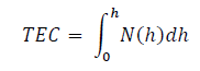 Equation 1
Along with the study of GPS TEC the present work also concern with the critical frequency of the F2 layer (foF2) as foF2 and TEC are the two important ionospheric parameters widely used by researchers for the investigation of spatial and temporal variations in the ionosphere [1,8-10]. It is very important to monitor these two parameters for the reliable operations of HF communications and GPS. The F2 layer of the ionosphere has been always directed to large variability and is always difficult for the space weather community to suggest reliable frequency for HF communication at this altitude.
The international reference ionosphere (IRI-2016) is an empirical model sponsored by the Committee on Space Research (COSPAR) and the International Union of Radio Science (URSI). This empirical model is widely used by the ionospheric community since its inception in 1070s to calculate the ionospheric parameters such as average electron density, electron temperature, ion temperature, ion composition, ion drift, electron content (TEC) and critical frequency of F2 layer etc. For a given time and location IRI-2016 can calculate the average electron density within the altitude range of 50 km to 2000 km. To calculate TEC and foF2, IRI-2016 is based on two different types of electron density maps i.e. URSI and CCIR. The user can select any one of these two maps to calculate foF2 and TEC.
NeQuick 2 is the latest version of the NeQuick ionosphere electron density model developed at the Aeronomy and Radioprpagation Laboratory (now T/ICT4D Laboratory) of the Abdul-Salam International Centre for Theoretical Physics (ICTP) – Trieste, Italy with the collaboration of the Institute for Geophysics, Astrophysics and Meteorology of the University of Graz, Austria. This model calculates the electron content through source code in FORTRAN language. The model uses the altitude range from starting point 50 km to ending point 20000 km. The user also has option to select starting and ending points of the integral. The user can retrieve electron content by mentioning location for given month and year. The output of the model contains data in simple text formats. The NeQuick model is based on the CCIR (Consultative Committee on International Radio) coefficients. The NeQuick model is widely used in GNSS (Global Navigation Satellite Systems) applications. In space weather the NeQuick model can provide realistic descriptions of the electron density of the ionosphere.
In this study, we present the diurnal and seasonal variations in GPS TEC along with its comparison with IRI -2016 TEC and NeQucik TEC at low latitude stations Sonmiani (magnetic lat: 17.34° N, long: 141.12° E) during HSA period of 2014-2015. Based on the smoothed sunspot number (SSN) index the period from May 2014 to September 2015 can be considered a HSA period. Among all local stations in Pakistan, Sonmiani has greatest effect of EIA. The observed TEC has been compared with IRI – 2016 TEC and NeQuick TEC to see the deviations in predictions of both ionospheric models. The GPS TEC ingested NeQuick foF2 has also been compared with IRI – 2016 foF2. A FORTRAN code iterative method is devised to obtain the Optimistic foF2 values by using GPS TEC data. These values are then compared with corresponding IRI-2016 foF2 to check the validity of iteration process. The Optimistic foF2 values are compared with IRI-2016 foF2 because of the unavailability of ionosonde foF2 for the same time duration.
Materials and Methods
The GPS TEC data is obtained from GPS receiver with 1 hour time interval so that 24 values are obtained for one day. The monthly average values are then calculated as median values for each specific hour i.e. 24 medians for each month. The GPS TEC data were available from May 2014 to September 2015. The correlation between GPS TEC and IRI-2016 TEC has been calculated by using Pearson’s Correlation Coefficient. Similarly the correlation between GPS TEC and NeQuick TEC has been calculated via same statistical tool. The Coefficient of Variability (CV) in monthly medians of GPS TEC has been calculated to check the variability. CV can be used as variability index in foF2 and TEC [7]. The CV in percentage is given by
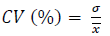 Equation 2
Where σ represent standard deviation and  represent mean.
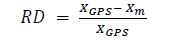
The statistical too Relative Deviation (RD) has been used to determine the deviation of IRI-2016 and NeQuick TEC from GPS TEC. RD has been used by several researchers [7] to study the model predictions.
 Equation 3
Where XGPS and Xm represent GPS TEC and model TEC respectively.
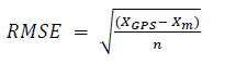
The Root Mean Square Error (RMSE) is a meaningful statistical test to analyse the discrepancy between observed and model data. Several researchers used RMSE in the field of ionosphere to explore the performance of IRI and NeQuick2 model for the prediction of two important ionospheric parameters fof2 and TEC [11-13].
The RMSE is given by
 Equation 4
Where XGPS and Xm represent GPS TEC and model TEC respectively and n represent number of observations.
The NeQuick model is used to calculate foF2 by ingesting GPS TEC. NeQuick can be made to execute such that it estimates foF2 by taking the GPS TEC as input. The NeQuick TEC and GPS TEC are also compared to obtain the correlation between model and observed values. In the present work the difference between NeQuick foF2 and IRI – 2016 foF2 is denoted by ΔfoF2 while ΔTEC represent the difference between NeQuick TEC and GPS TEC. This difference is considered as good point if less than ±1 MHz otherwise it is considered as a bad point. The NeQuick model uses FORTRAN code to retrieved average electron density, foF2, TEC and slab thickness etc. In order to obtain NeQuick model data the date and geographical coordinates will have to be mention in the program. This model also contains the package in which experimental data for any parameter can be given as input to the model. In this work the GPS TEC is used as input parameter to the NeQuick code for the estimation of foF2 and the output foF2 is name as GPS TEC ingested foF2 i.e. the topside ionosphere information predicted by the model would not be apply.
Results and Discussions
Correlation between GPS TEC and IRI-2016 foF2
The GPS TEC and IRI – 2016 foF2 shows high correlation coefficient between them and most of the time coefficients are greater than 0.95 as shown in TABLE 1. The strong correlation exists between GPS TEC and model foF2.
| Correlation Coefficients | ||||
|---|---|---|---|---|
| GPS TEC and IRI ? 2016 TEC | GPS TEC and IRI ? 2016 foF2 | |||
| Month | 2014 | 2015 | 2014 | 2015 |
| Jan | - | 0.94 | - | 0.92 |
| Feb | - | 0.96 | - | 0.96 |
| Mar | - | 0.97 | - | 0.96 |
| Apr | - | 0.97 | - | 0.97 |
| May | 0.96 | 0.98 | 0.96 | 0.99 |
| Jun | 0.93 | 0.93 | 0.96 | 0.95 |
| Jul | 0.97 | 0.98 | 0.98 | 0.99 |
| Aug | 0.99 | 0.94 | 0.98 | 0.98 |
| Sep | 0.98 | - | 0.96 | 0.92 |
| Oct | 0.99 | - | 0.97 | - |
| Nov | 0.96 | - | 0.94 | - |
| Dev | 0.95 | - | 0.93 | - |
Table 1: Correlation between GPS TEC and IRI- 2016 foF2 and TEC.
Similarly the correlation coefficients between GPS TEC and IRI-2016 TEC have been calculated for the same period and it is found that most of the time coefficients are greater than 0.95. It has also been observed by other researchers that strong correlation exist foF2 and TEC [1,2]. The monthly maximum values of GPS TEC and IRI-2016 foF2 are shown in FIG. 1 while the monthly maximum values of GPS TEC and IRI – 2016 TEC are shown in FIG. 2.

Figure 1: Comparison between monthly maximum values of GPS TEC and IRI-2016 foF2 during May 2014 - September 2015.

Figure 2: Comparison between monthly maximum values of GPS TEC and IRI-2016 TEC during May 2014-September 2015.
Diurnal variations in GPS TEC
The diurnal variations in GPS TEC have been analysed and it has been observed that most of the time the peak value of the day is observed during 1500LT and the minimum value is observed during sunset and pre-sunset hour’s i.e.0000LT-0600LT. The highest peak value is observed in April 2015 (around 80 TECU). The peak value around post noon hour shows the maximum ionization in the ionosphere due to the solar radiation take some time after noon hour at low solar zenith angle. The sharp gradients are observed in diurnal variations of GPS TEC during the sunset and sunrise hours. These gradients are due to the abrupt change in solar radiations around sunrise and sunset. The diurnal variations in GPS TEC during 2014 and 2015 are shown in FIG. 3 and 4 respectively.

Figure 3: Diurnal variations in GPS TEC during HSA year 2014.

Figure 4: Diurnal variations in GPS TEC during HSA year 2015.
Seasonal anomaly or winter anomaly
Seasonal anomaly is observed in GPS TEC with reasonable amplitude during both the years 2014 and 2015. The monthly medians of GPS TEC in June and December have been compared to see the winter anomaly. The monthly medians of GPS TEC in December solstice of the year 2014 have been compared with both the June solstice of the years 2014 and 2015. It can be seen very clearly that the TEC values in December are larger than the TEC values observed in June. This difference is realistic around noon hours.
In the year 2014 the TEC value observed in June at 1600LT is around 36 TECU while at the same LT the TEC value observed in December is around 49 TECU. The difference is around 15 TECU. In the year 2015 the TEC value observed in June at 1600LT is around 38 TECU while at the same LT the TEC value observed in December is around 47 TECU. The difference is around 9 TECU FIG. 5.

Figure 5: Winter anomaly in GPS TEC during 2014 and 2015.
The difference between peak values in December solstice and June solstice shows the amplitude of winter anomaly. It can be seen very clearly while proceeding from the year 2014 to the year 2015 that the amplitude of winter anomaly decreases. The year 2014 is relatively HSA year as compared to the year 2015. In general we can say that amplitude of winter anomaly is decaying with decrease in solar activity. This result is also supported by [1,14-16]. Also the winter anomaly is only observed during the daytime while it is completely absent during the nighttime. The winter anomaly arises due to dissimilar variations in atomic to molecular constituents in neutral atmosphere [16]. The atomic to molecular ratio in the neutral atmosphere is thought to be the basic source of winter anomaly.
Semi-annual variations
The semi-annual variations in GPS TEC have been analysed during HSA period from May 2014 to September 2015. It has been observed that the GPS TEC show high values during equinoctial months i.e. during September 2014 and April 2015 and lowest values during June solstice of both the years 2014 and 2015. The highest peak value of TEC monthly medians is observed during the September 2014 at 1500LT which is around 75 TECU. The lowest values are observed during the June 2014 which has peak value at 1500LT around 38 TECU. Similarly in the year 2015 the highest value in GPS TEC observed in April at 1500LT is around 80 TECU. The lowest peak value at 1500LT is observed in June solstice which is around 40 TECU. The GPS TEC reaches up to 84 TECU in April 2015 and up to 74 TECU in September 2014. The monthly medians of GPS TEC show a difference of around 40 TECU between equinoctial months and solstice months. In general it can be said that the semi-annual variations are clear at low latitude station Sonmiani showing high values in equinoctial months as compared to solstice months. Semi-annual variations are one of the features of EIA region and that is why it shows strengthening at low latitude station Sonmiani. Several researchers show semi-annual variations in different time durations [14,17,18]. It has been suggested that semi-annual variations in neutral densities of the atmosphere associated with geomagnetic and aurora activity are the sources of semi-annual trends in the ionosphere [16] FIG. 6.

Figure 6: Seasonal variations in GPS TEC during the period of HSA 2014-2015.
Coefficient of Variability (CV) in GPS TEC
To analyse the variability in GPS TEC the coefficients of variability have been found in the year 2014 and 2015. The coefficients of variability have been found relatively greater in 2015 as compared to 2014. It can be seen in the following table that the coefficients of variation are small in June solstice as compared to other months as December solstice and equinoctial months. In general the GPS TEC shows high variability in winter and equinoctial months. The large CV in GPS TEC is due to the reason that TEC is also affected by topside ionosphere which has completely different electrodynamics as compared to bottom side ionosphere. There might be some other sources of variability in TEC e.g. neutral winds, compositional changes and equatorial fountain affects [2]. The CV in percentage is given in TABLE 2.
| CV(%) in GPS TEC | ||
|---|---|---|
| Month | 2014 | 2015 |
| Jan | - | 72.81 |
| Feb | - | 69.59 |
| Mar | - | 66.87 |
| Apr | - | 56.66 |
| May | 45.37 | 49.00 |
| Jun | 40.54 | 39.22 |
| Jul | 52.94 | 51.55 |
| Aug | 60.86 | 53.64 |
| Sep | 48.00 | 72.15 |
| Oct | 48.00 | - |
| Nov | 63.50 | - |
| Dec | 66.09 | - |
Table 2: CV in monthly medians of GPS TEC during 2014-2015.
The IRI-2016 TEC has been compared with the GPS TEC. It has been observed that the correlation between GPS TEC and IRI-2016 TEC is greater than 0.9. The comparison between GPS TEC and IRI – 2016 TEC during the year 2014 can be seen in FIG. 7 and 8. The GPS TEC and IRI – 2016 TEC shows good agreement around September equinox and December solstice as compared to June solstice. Similarly the comparison between GPS TEC and IRI – 2016 TEC during the year 2015 can be seen in FIG. 9 and 10. The GPS and IRI – 2016 TEC shows good agreement in the month of July otherwise disagreement can be seen in other months.

Figure 7: Comparison between GPS TEC and IRI-2016 TEC during 2014.

Figure 8: Relative deviations in IRI ? 2016 TEC during the year 2014.

Figure 9: Comparison between GPS TEC and IRI-2016 TEC during 2015.

Figure 10: Relative deviations in IRI ? 2016 TEC during the year 2015.
The deviation of IRI-2016 TEC form GPS TEC is large during daytime as compared to nighttime. The relative deviations are large during equinoctial months as compared to solstice months. The sharp gradient in the relative deviations has been observed around 0500LT.High discrepancies are observed around 0800 – 1000 LT and 1800 – 2300 LT. It has been also revealed [11] at equatorial region Ethiopia during 2009 and 2013. During LSA year 2009 high discrepancies were found between 0800 – 1100 LT and 1800 – 2300 LT. During HSA year 2013 high discrepancies were found between 0800 – 1100 LT, 1200 – 1800 LT and 1800 – 2300 LT.
The deviation of IRI-2016 TEC from GPS TEC has been found greater in relatively HSA year 2014 as compared to 2015. It can be suggested as the direct impact of the fact that the variability in TEC is greater in the year 2015 as compared to 2014. It can be seen in the FIG. 8 and 10 that the relative deviations show slender trend in 2015 as compared to 2014.
The year 2014 is comparatively HSA as compared to 2015. In general, the IRI – 2016 predictions are relatively better in 2015. It has been found that the IRI model performs better during LSA 2008 and 2009 in East African equatorial stations [19].
IRI - 2016 foF2 and GPS TEC ingested foF2
The IRI – 2016 foF2 and GPS TEC ingested NeQuick foF2 are plotted in FIG. 11 during the years 2014 and 2015. In general, both datasets of foF2 shows good agreement. There are some discrepancies around June solstice in the year 2014.

Figure 11: Comparison between IRI ? 2016 foF2 and GPS TEC ingested NeQuick foF2.
The results are relatively better during the year 2015. It can be seen in figure that IRI - 2016 foF2 and GPS TEC ingested NeQuick foF2 shows good agreement around September equinox and December solstice.
Iterations for the determination of optimistic foF2
The iteration process to determine optimistic foF2 from GPS TEC has been performed for Sonmiani during the period (May 2014 to September 2015). The model foF2 is compared with TEC ingested foF2 and the difference of two frequencies is denoted by ΔfoF2. The iteration is performed for total 408 monthly medians.
If the obtained foF2 value lies within ± 1MHz tolerance then it is considered as good point i.e. the obtained foF2 value will be hopeful. The result of the iteration process is shown in the following TABLE 3.
| Year | Months | ΔfoF2 ≤ MHz | ΔfoF2 = 0 | Total Points |
|---|---|---|---|---|
| 2014 | May - December | 129 (67.20%) | 32 (16.70%) | 192 |
| 2015 | January - September | 155 (71.75%) | 34 (15.74%) | 216 |
| Total | 284 (70%) | 66 (16.17%) | 408 |
Table 3: Result of Iteration process.
The 70% of the total data results into a tolerance level of ± 1MHz and 16.17% of the total values gives ΔfoF2 equal to zero. In table it can be seen very clearly that the results are quiet better in the year 2015 which is LSA year as compared to 2014 (FIG. 12).

Figure 12: The spread of ΔfoF2 in iterations results.
The iteration process show interesting results at Sonmiani that the 70% points gives tolerance equal to less than or equal to 1 MHz also the 17% of the total iteration show delta foF2 equal to zero MHz. The same exercise was performed at Vanimo (Geog. Lat: 2.7°S, Long: 142.00°E) for May 2007 [1].
The iterations were performed for total 398 points of the month. The numbers of good points were 225 out of 398 (56.54%).
Root Mean Square Error (RMSE) in IRI-2016 TEC
The root mean square error (RMSE) in IRI – 2016 TEC and NeQuick TEC are calculated and mentioned in TABLE 4. The lowest RMSE observed in IRI – 2016 TEC is 2.64 in July 2015 while the highest RMSE observed in the same TEC is 17.26 in May 2014. Similarly the lowest RMSE observed in NeQuick TEC is 1.38 in August 2015 while the highest RMSE observed in the same model TEC is 23.95 in March 2015.
| RMSE in TEC | ||||
|---|---|---|---|---|
| IRI-2016 TEC | NeQuick TEC | |||
| Month | 2014 | 2015 | 2014 | 2015 |
| JAN | - | 5.26 | - | 4.19 |
| FEB | - | 8.13 | - | 16.78 |
| MAR | - | 11.86 | - | 23.95 |
| APR | - | 9.26 | - | 14.15 |
| MAY | 17.26 | 5.36 | 15.11 | 1.63 |
| JUN | 10.67 | 6.20 | 6.41 | 2.55 |
| JUL | 7.10 | 2.64 | 3.88 | 4.99 |
| AUG | 4.10 | 5.96 | 4.20 | 1.38 |
| SEP | 6.20 | 9.60 | 6.73 | 8.521 |
| OCT | 3.88 | - | 6.88 | - |
| NOV | 4.95 | - | 5.43 | - |
| DEC | 4.95 | - | 5.24 | - |
Table 4: RMSE in IRI - 2016 TEC and NeQuick TEC.
In general, the RMSE in NeQuick TEC shows larger values as compared to IRI – 2016 TEC. It can also be seen in the TABLE 4 during the period May 2014 - September 2015 the RMSE values are comparatively higher in equinoctial months. This result is supported [12] at equatorial station Ilorin (Geog. Lat. 8.50°N, Long. 4.50°E, dip -7.9°) during the year 2010.
Conclusions and Suggestions
1. Strong positive correlation exists between model foF2 and GPS TEC i.e. greater than 0.95 most of the time
2. Winter anomaly exists during the period with relatively large amplitude during HSA year 2014
3. The GPS TEC shows strengthen in seasonal variations with higher values at equinoctial month as compared to solstice months
4. The diurnal variations in GPS TEC show peak value around post noon hour i.e. 1500LT
5. The relative deviation in IRI-2016 TEC has been found large during 2014
6. The model shows discrepancies between 0800 – 1000 LT and 1800 – 2300 LT with peak deviation around 0500 LT
7. The 70% of the total data results into a tolerance level of ± 1MHz and 16.17% of the total values gives ΔfoF2 equal to zero. The optimistic foF2 values can be found with more confidence if continues GPS TEC data is available
8. The iteration results can be further improved if we use continuous GPS TEC data and for this more GPS receivers are required to be installed at different locations in Pakistan
Acknowledgement
The author is very thankful to the Manager of Space Weather Monitoring (SWM) division of SUPARCO (Pakistan Space and Upper Atmospheric Research Commission), Mr. Ayaz Ameen for his great support. The FORTRAN based program code for iteration process and the GPS TEC data for Sonmiani have been provided by him. The TEC data is obtained from GPS TEC receiver setup at Sonmiani by SUPARCO in collaboration with China Research Institute of Radiowave Propagation (CRIRP). The author is thankful to the Dr. Naeem Sadiq, Assistant Professor at ISPA (Institute of Space and Planetary Astrophysics) University of Karachi for helping in writing skills of research paper. This work is the part of collaboration between University of Karachi and SUPARCO. The SUPARCO and University of Karachi collaboration is very effective in the past few years. The author is also very thankful to the Director of Institute of Space and Planetary Astrophysics (ISPA), Dr Jawed Iqbal and Chairman SUPARCO, Major General Qaiser Anees Khurram who provides this opportunity for research work.
References
- Ameen MA. A study of the relationship between the Critical Frequency of the F2 - layer of the Ionosphere and the GPS Total Electron Content in the Equatorial Anomaly region. 2011.
- Saranya PL, Prasad DSVVDK, Niranjan, et al. Short term variability in foF2 and TEC over low latitude stations in the Indian sector. Ind J Radio and Space Physics. 2015;44:14-27.
- Pietrella M, Pezzopane M, Scotto C.Variability of foF2 over Rome and Gibilmanna during three solar cycles (1976 -2000). J Geo-Phy Res. 2012;117:A05316
- Gnabahou DA, Ouattara F, Nanema E, et al. foF2 Diurnal Variability at African Equatorial Stations: Dip Equator Secular Displacement Effect. Int J Geosci. 2013;4:1145-1150
- Mosert M, Ezquer R, Jadur C, et al. Time variation of total electron content over Tucuman, Argentina. Geofisica Int. 2004; 43:143-151.
- Sharma N, Dabas RS, Pillaii MGK, et al. A multi-station satellite radio beacon study of ionospheric variations during total solar eclipses. J Atmos Terr Phys. 1989.
- Akala AO, Somoye EO, Adeloye AB, et al. Ionospheric foF2 variability at equatorial and low latitudes during high, moderate and low solar activity. Ind J Radio and Space Phys. 2011;40:124-129
- Muslim B, Haralambous H, Oikonomou C, et al. Evaluation of a global model of ionospheric slab thickness for foF2 estimation during geomagnetic storm, Ann Geophys. 2015;58:A0551
- Kenpankho P, Supnithi P, Tsugawa T, et al. Variations of ionospheric slab thickness observations at Chumphon magnetic equatorial location. Earth Planets Space. 2011;63:359-364
- Krankowski A, Shagimuratov II, Baran LW. Mapping of foF2 over Europe based on GPS-derived TEC data. Adv Space Res. 2007;39:651-660.
- Asmare Y, Kassa T, Nigussie M. Validation of IRI-2012 TEC model over Ethiopia during solar minimum (2009) and solar maximum (2013) phases. Adv Space Res. 2014;53:1582-1594
- Adebiyi SJ, Adimula IA, Oladipo OA, et al. GPS derived TEC and foF2 variability at an equatorial station and the performance of IRI - model. Adv Space Res. 2014; 54:565-575.
- Kenpankho P, Supnithi P, Nagatsuma T. Comparison of observed TEC values with IRI-2007 TEC and IRI-2007 TEC with optional foF2 measurements predictions at an equatorial region, Thailand. Adv Space Res. 2013; 52:1820-1826.
- Mosert M, Mckinnell LA, Gende M, et al. Variations of foF2 and GPS total electron content over the Antarctic sector. Earth Planets Space. 2011;63; 327-333
- Kumar S, Singh AK, Lee J. Equatorial Ionospheric Anomaly (EIA) and comparison with IRI model during descending phase of solar activity (2005-2009). Adv Space Res. 2014.
- Torr DG, Torr MR. The seasonal behavior of the F2 layer of the ionosphere. J Atmos Terr Phys 1973;35:2237-2251
- Bhonsle RV, Da Rosa AV, Garriott OK. Measurement of the total electron content and the equivalent slab thickness of the mid ? latitude ionosphere. Radio Sci. 1965;69:929-937
- Hunsucker RD, Hargreaves JK. The high latitude ionosphere and its effect on radio propagation. Cambridge University Press, 2003.
- Nigusse M, Radicella SM, Damtie B, et al. Validation of the NeQuick2 and IRI-2007 models in East-African equatorial region. J Atmos Solar Terr Phys. 2013;102:26-33.