Research
, Volume: 12( 1) DOI: 10.37532/2320-6756.2023.11(4).337Statistical Independence in Quantum Mechanics
- *Correspondence:
- John P. Wallace
Casting Analysis Corp., 8379 Ursa Lane, Weyers Cave, Virginia 24486 USA
E-mail: jpw@castinganalysis.com
Received date: 10-April-2023, Manuscript No. tspa-23- 95037; Editor assigned: 13-April-2023, PreQC No. tspa-23-95037 (PQ); Reviewed: 21- April-2023, QC No. tspa-23-95037 (Q); Revised: 23-April-2023, Manuscript No. tspa-23-95037 (R); Published: 28-April-2023, DOI. 10.37532/2320-6756.2023.11(4).337
Citation: Wallace J.P. Statistical Independence in Quantum Mechanics. J. Phys. Astron.2023;11(4):337.
Abstract
Algebraic mistakes of using a non-relativistic functions betrayed Dirac’s elegant derivation of the relativistic equation of quantum mechanics and exposed a short coming of special relativity. It was a serious mistake because that famous paper became a model for theorist to follow who produced an unending stream of nonsense. The mistake was compounded because it hid the fact that special relativity was still incomplete. Multiple independent spaces are required to generate both dynamics as well as produce particle properties. The concept of statistical independence of spaces that encapsulated quantum objects, fields and particles, was necessary for physics to have a relativistic basis for both massive particles and massless fields. The example that will be developed is the origin of the solar neutrino survival data that requires the electron neutrino to be massless as originally proposed by Pauli. The analysis renders a proof of the original quantum conjecture by Planck and Einstein that radiation is quantized and how inertia for massive particles is generated.
References
Blog | Real Estate in Australia Blog | Real Estate in Germany Car Insurance in USA Blog | Real Estate in Greece Casino Sites in Indonesia Blog | Real Estate in Indonesia Find Lawyer in Virginia Blog | Real Estate in India Casino Sites in India Blog | Real Estate in Malaysia Find Lawyer in Utah Blog | Real Estate in Philippines Best Betting Sites in Australia Blog | Real Estate in UK Casino Sites in Ethiopia Blog | Real Estate in USA Find Lawyer in Texas Blog | Real Estate in Croiatia Blog | Real Estate in Balkans Blog | Real Estate in BrazilKeywords
Quantum mechanics; Relativity; Neutrinos
Introduction
The foundation of quantum mechanics suffers a number of defects. Two defects in the subject are the missing mechanism that quantizes the massless fields and generation of inertia or the self-energy of massive particles. A third problem that has not been resolved is the generation of static potentials and that is key to understanding material properties. Einstein introduced special relativity in 1905 and went on to produce general relativity, however, special relativity had not been completed as was guessed by J.S Bell [1]. When in 1928 Dirac introduced his relativistic equation for quantum dynamics, both Einstein and Dirac ignored the physical implications of the quadratic form of the relativistic energy conservation relation, equation. 3, and their work after that point ceased to be significant.
Physical statistical independence is a quantum concept. Our introduction to the concept came through Mark Kac, who continued a very productive line of research after studying diffusion and Brownian motion [2, 3]. In the late 1940s his work was subsequently used in a quantum description of nonrelativistic path integral analysis that looked much like diffusion. Kac’s work was a help in understanding the quantum diffusion of hydrogen and its isotopes in metals, particularly iron. The question arose: What is the minimum potential well depth supporting a bound state? The answer in three dimensions yields a very curious result. This minimum bound state for a vanishingly small potential well for a particle produces the Compton relation independent of the potential wells depth and only dependent on the potential well’s radius [4]. This is a limiting case application of the Schrödinger equation begins to expose the source of an inertial mass.
In the middle of the 1960s, Kac posed another interesting problem relevant to those trying to understand high energy scattering data to work out the structure of nucleons [5]: Can one hear the shape of a drum with holes? If you beat on an arbitrary drum will its audible spectrum contain enough data to accurately reconstruct the drum? The symbolism of an excited drum head might strike his physics colleagues as something familiar. In the 1950s Kac’s mathematical interests were applied to discrete random processes and the concept of statistical independence of random variables [6].
The random walk generated by Brownian motion was a nice analogy but not physically realistic for fleshing out the statistical basis of quantum mechanics. The nonrelativistic path integral approach that Kac was exploring with Feynman was an attack on the dynamic problem of quantum objects; unfortunately, their elementary particles entered in as Newtonian point masses and point charges. The fields entered in as plane or spherical waves. These assumptions removed consideration of the particle/field structure as relativity did not make it into the analysis. Kac’s consideration of a defective drum made the particle a real structure. The scale of the drum head removes the point particle assumption as a barrier to having a particle with a defined scale. The complex spectra of the drum was a start at producing a basis for a scattering particle’s properties and immediately brought into question the completeness of the information content of the spectra.
Kac, with his drum analogy, was able to take the problem to a lower level and in a different direction by showing that the inversion techniques operating on the measured spectral output fails to determine the true structure of the drum because that requires more data than can ever be collected. Kac’s failed inversion analysis highlights the high energy potential scattering problem that of determining an unknown potential’s structure by scattering experiments such as done with accelerators.
The Lowly Potential
The Schrödinger equation, matrix mechanics, Klein Gordon equation, and the Dirac equation were impediments to discovering the structure of particles and fields. The legacy opposition to exploring the structure of elementary particles and fields was strengthened by theorists developing quantum electrodynamics and the effective field theories for high energy. The reason for this was simple, they embraced a method to rid themselves of having to explain the electrostatic potential and other force potentials. This was accomplished by assuming there was an exchange boson, a gauge field, to explain each and every force: electromagnetic, gravity, strong and the weak force. This was a terrible mistake and its origin was in the failed attempts at explaining the origin of inertia. The point mass and point charge of the 18th, 19th, and 20th century were useful tools and to abandon them meant also abandoning the conveniences of the mathematical continuum.
To have a potential independent of an exchange boson it was necessary for the particle to have a structure, beyond that of point mass. Kac’s drum head with holes illustrates the failure of high energy experiments to yield the structure of an elementary particle. The myth that high energy accelerator experiments function as a high resolution microscope of structure was exposed and ignored. In order to experimentally crack the problem, quantum mechanics itself provides the assistance if examined at low energy. Quantum structures scale from elementary particle to collections of particles behaving with simple quantum properties such as superconducting currents and magnetic excitation. These large low energy structure are more easily explored by experiment.
Exposing the Self-Reference Frame
Instead of the acoustical problem that Kac posed, the problem was recast into one of a near-field electromagnetic scattering problem using multiple simultaneous frequencies to examine an unknown object’s: range, scale, conductivity, and magnetic permeability [7]. Maxwell’s equations can be solved explicitly for the forward problem, and checked against known materials [8]. It was found that when unknown materials are used their conductivity and permeability properties can be accurately extracted if they behave with the following two material constitutive restrictions.
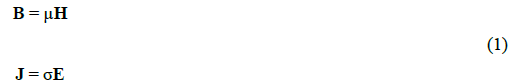
From the solutions of the forward problem the domain of allowed solutions can be determined and the allowed reflection responses are defined by the restrictions found in equation. 1[9]. This is no different than a photon mediated high energy scattering problem. As long as these conditions are in place a rough inverse problem can be solved to the precision of the measurements and produce useful information. However, the inverse analysis, analogous to Kac’s drum problem, fails spectacularly if the material is capable of absorbing the incoming energy and processing it into an excited quantum state on the scale of the object being examined. The object then becomes Kac’s drum head, where the holes in the drum form a spectrum of their own not described by the Faraday-Maxwell equations.
For the transverse electromagnetic problem the Faraday-Maxwell description now needs to be extended, but there is not much in the
scattering data to tell one how to accomplish this task when done in well annealed iron or a low carbon steel. To measure the field’s
properties an experiment must be done to capture the dispersion relations of the newly observed fields. The new data acquired resolved
a longitudinal field with an effective mass very different from the original massless transverse fields [10 , 11]. The dispersion relation
for a well annealed iron or a low carbon steel is actually more complex producing three fields with the most interesting, a propagating
field, with a mass of 10-9 of an electron’s mass. This very light spin wave involving the two electron spin bands has a correspondingly
large scale  meters. A low frequency magnetic field drives the creation of an exciton that is an oscillating longitudinal
magnetization wave with mass and large scale structure. This solved a major experimental problem because now a quantum particle
structure can be examined in detail on a lab bench. It turns out this particle is a spin zero boson and not a fermion. A Bose-Einstein
condensate can form at temperatures that exceed the Curie point of the metal because of its low mass making it even easy to study
over a wide temperature range. This light exciton must be treated from the beginning as a relativistic particle because of its small
mass [12].
meters. A low frequency magnetic field drives the creation of an exciton that is an oscillating longitudinal
magnetization wave with mass and large scale structure. This solved a major experimental problem because now a quantum particle
structure can be examined in detail on a lab bench. It turns out this particle is a spin zero boson and not a fermion. A Bose-Einstein
condensate can form at temperatures that exceed the Curie point of the metal because of its low mass making it even easy to study
over a wide temperature range. This light exciton must be treated from the beginning as a relativistic particle because of its small
mass [12].
Energy Conservation
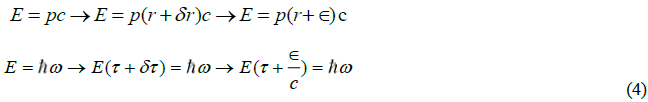
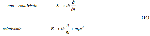
To discover how inertia is produced for this magnetic excitation energy conservation relation must be examined. Quantum mechanics and relativity were discovered almost together in 1900-1905. They were treated as separate subjects, because the connections between the two was unknown. Both fields were forced into a mold that mirrored classical mechanics and this further separated the fields making both subjects even more opaque. Starting with the tested conservation of energy expressions for a massless field and a massive particle where mo is the rest mass the role of the relativity becomes clear.
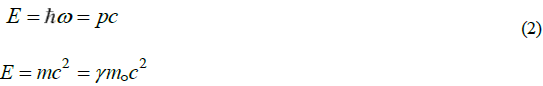
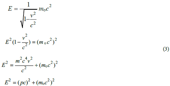
Einstein use mc2 form of mass energy relation in his publications Relativity but Dirac used the square root of the expression as his model containing momentum to derive his relativistic equation. In Einstein’s book the expression containing momentum does not appear and first appears in Dirac’s paper. The quadratic expression was a problem for both Einstein and Dirac. For Einstein the problem was that the two energies were not simply additive as in thermodynamics. For Dirac, the problem was also the quadratic, as he also wanted a linear relation in energy for his relativistic model. This prejudice against a second order energy relation was unwarranted and help stall the development of quantum mechanics and physics as a whole.
Classical non-relativistic quantum mechanics approximates two problem well: the hydrogen atom and the harmonic oscillator. It does not accurately handle the free particle, along with diffraction, refraction, pair production, nor generate the general description of quantum particles: boson and fermion. This collection of defects reflect a poor understanding the two energy conservation relations.
There is a myth that quantum electrodynamics, a method of calculation, has made quantum mechanics the most accurate theory ever. Quantum electrodynamics non-unique set of corrections are considered even by R. Feynman, one of the originators, not a description of physics, but a method of calculation. The non-uniqueness allows result to use non-physical properties (potentials with singularities) to generate any desired number. Whereas, the two empirical conservation of energy relations, equation 4 and equation 3, allows one to derive a description of the space where particle and field properties are generated, the self-reference frame, and their subsequent behavior in the laboratory frame. This requires a two part derivation to generate both structure and dynamics in two separate spaces. These spaces are not in hierarchy, but complimentary where each space’s existence is dependent on the other.
Self-Reference Frame
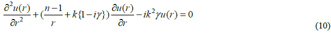
Starting with the massless field conservation of energy and randomizing motion for that field begins the derivation to produce structure and inertia. This randomizing process is generated independently when the dynamic equation is derived in the next section. The particle’s structural form in the space referenced on the particle itself can be generated by Taylor expanding the momentum and energy operators around r and r of the field with the random spatial parameter ∈, and time parameter c/ ∈ resulting in two differential equation, one for the spatial structure, u(r) , and one for the time dependence, g(τ) , which are derived in detail. The derivation begins with the expansions:
The entire concept of a point mass and point charge with their associated infinite energies vanish in this picture along with the cut offs necessary in quantum electrodynamics. What also vanishes is the single virtual photon, which cannot be supported because it will change the information content of the laboratory frame.
Starting with the dispersion relation for a massless field in laboratory frame [14]:

The spatial dependent equation will be derived first where u(x) is the spatial dependent function by applying the momentum operator.

The scale of uncertainty in space,∈, enters the spatial equation as a random offset that is greater than zero. In the spatial differential equation becomes a second order differential equation.

The result of expanding the differential forms of the dispersion relation with the disorder parameters is a pair of differential equation for the spatial variable, r , the radial coordinate and the time coordinate,τ . Access to the angular coordinates in spherical geometry are lost in the random behavior introduced to generate a particle description located on the instantaneous center of symmetry of the particle.
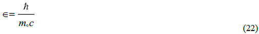
Using the Compton scattering particle scale parameter for ∈ gives it a value of  The field equation are written in terms
of the dimension of space, n , with the parameters
The field equation are written in terms
of the dimension of space, n , with the parameters  The resulting spatial differential
equation from expanding the conservation of energy relation and referenced to the particles instantaneous center of symmetry.
The resulting spatial differential
equation from expanding the conservation of energy relation and referenced to the particles instantaneous center of symmetry.
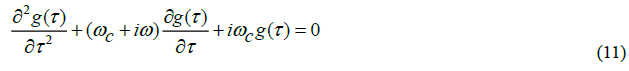
The time dependent equation can also be expanded from the dispersion relation  with the use of the energy operator for a
massless field.
with the use of the energy operator for a
massless field.
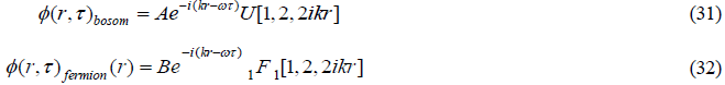
The second order spatial equation has two solutions that include the confluent hypergeometric functions 1F1 and U where A and B are constants [15]:
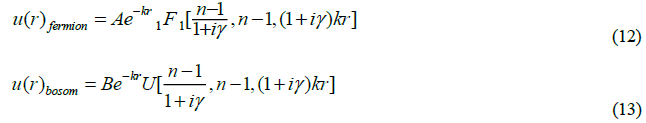
What was discovered on inspecting these two solutions were properties consistent with the two families of particles with mass: boson
and fermion [12]. The first solution represents a fermion and the second solution represents a boson both with a real mass. All
densities determined from the solutions retain spherical group symmetry,U(1) . In three dimensions the function u*(r)u(r) is used
to directly define the particle’s static field. This field defines the particle’s structure. Charge density can then be computed from
Gauss’s law if particle can support a charge [14]. This generates the charge radius of the particle. The charge quantization for
fermions can be determined by an analysis of the derivative  For the massive fermion this will produce a quantized charge,
mass independence of charge, and the dimensional dependence of charge where θ is the argument of u(r) on the complex plane:
For the massive fermion this will produce a quantized charge,
mass independence of charge, and the dimensional dependence of charge where θ is the argument of u(r) on the complex plane:  If there is no θ dependence in u(r) the particle has a zero charge and cannot support an
electromagnetic transition [12].
If there is no θ dependence in u(r) the particle has a zero charge and cannot support an
electromagnetic transition [12].
The self-reference frame also allow the anti-particles to be described as γ can take on a negative value [14]. The anti-particle
function,  have the opposite rotational symmetry, right and left handed spirals on the complex plane differentiate to two types. In
addition it was found that | γ | can take on values less than one when the particle is in a bound state [16]. These are extensions to
special relativity that are essential in developing material properties.
have the opposite rotational symmetry, right and left handed spirals on the complex plane differentiate to two types. In
addition it was found that | γ | can take on values less than one when the particle is in a bound state [16]. These are extensions to
special relativity that are essential in developing material properties.
The massive boson solution in three dimension, n = 3, shows a relative energy dependence through γ of the value of the u(r) at the origin that is not fixed as it is for the fermion, see FIG. 1. That is the source of CP violation expected for the massive 3D boson. The massive fermion solution in three dimensions has fixed value of u(r) at the origin with no CP problems. This has been extended to the analysis for baryons, proton and neutron, for which no CP problem were found and no need for the Axion [17].
This space, the self-reference frame, is a primitive domain where no form of momentum is defined and the dynamics only refer to the relative stability of the particles. The equations are compatible with relativity throughγ , which describes their behavior with different relative observers. Linear momentum, angular momentum, spin, and the magnetic moments are dynamic properties of the laboratory frame and are not part of the particle’s information developed in the self-reference frame. These properties are easily developed in the laboratory frame from the particle’s structure [17].
The importance of the self-reference frame is that as a statistically independent space it can generate the particle’s self-energy. Independence means there is no mapping between the two frames, either in space or time. This independence is reflected in the Pythagorean sum required for the two components in the conservation of energy relation, equation 3, which adds the square of the kinetic energy to the square of the self-energy. Rather than add physical dimensions to the 3+1 space of the laboratory frame for additional particles it is possible for any particle or collection of related particles to establish an embedded private space statistically independent from the laboratory frame and from other particles and fields. This forms the basis of true superposition with no extra assumptions.
Dirac in 1932 tried to reverse his course with an introducing a second order field equation and private time [18]. That ran into severe opposition from Pauli and Wessikopf who used a counter argument that involved the Klein-Gordon equation that does not conserve energy [19]. Not much had changed 26 years later in 1958 when Dirac had come out with the 4th edition of the text Quantum Mechanics he was still troubled, and quoting from the last paragraph of his book, “THE DIFFICULTIES BEING OF A PROFOUND CHARACTER, CAN ONLY BE REMOVED ONLY BY SOME DRASTIC CHANGE IN THE FOUNDATION OF THE THEORY,” [20]. The difficulties had to do with a series of infinities generated by the point particle description and his sea of negative energy positrons, neither of which are physically realistic.
Relativistic laboratory frame equation
Because of these errors the original Dirac equation was only partially relativistic and this showed up in the singularity at the origin of the 1S state of hydrogen at the origin [21]. The problem is more apparent in computing the ground state energy of high Z one electron ions. The values from the Dirac ground state energy closely tracked those of the Schrödinger equations, whereas, the behavior for the full relativistic ground state energy is very different [14]. A relativistic energy operator when applied in the laboratory frame not only has to support dynamics it also must include the particles self-energy. The relativistic energy operator, which is a first order time derivative plus the particle’s rest self-energy.
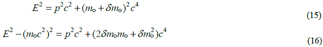
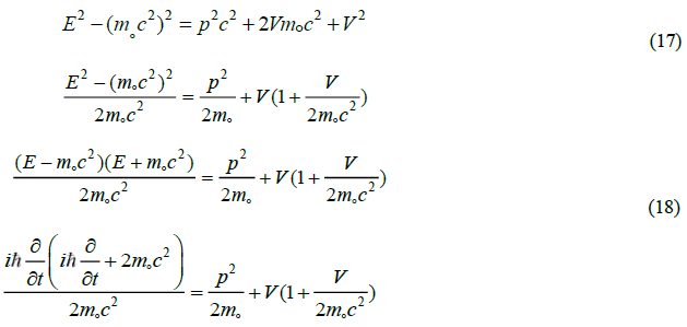
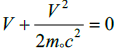
The second half of the derivation to compliment the self-reference frame properties requires generating the compatible dynamics in the laboratory frame. This automatically produces the mechanism that generates the basic statistical properties of quantum mechanics required by the self-reference frame. To do this the concept of a potential is necessary and now it is based on the structure of the particle itself as derived in the self-reference frame. Within the relativistic conservation relation the potential is derived from the mass of the particle. The variation m-mo= δmo reresents the energy source of the potential.
 is small relative to
  and is not dropped. The potential is taken to be
  producing an exact relativistic
expression containing the potential.
producing an exact relativistic
expression containing the potential.
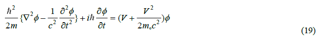
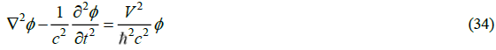
Using the momentum operator and the correct energy operator equation 3 is converted into the resulting differential equation, which has two additional terms absent from the Schrödinger equation. The second order time dependent term embedded the propagating field equation more commonly found from electromagnetic theory of Maxwell. The second addition is a quadratic term in the potential, whose presence brings in the mechanics of pair-production naturally [22].
The above equation can be reduced to the standard Schrödinger equation for some bound state and free propagation problems. This comes at a cost of losing its compatibility with relativity and the loss of the free field embedded wave equation. That reduction introduces a number of errors historically attacked by perturbation techniques.
The laboratory frame description of a massive particle yields the mechanisms of random behavior necessary to produce inertia, in the
quadratic term of the potential. When the potential contribution in free space with no external potentials there remain two solutions
to the above equation 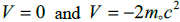 where both solutions are equally weighted. The second solution represent a pair
production allowed by the Heisenberg relation of particle and anti-particle the same as the original being described. The annihilation
with either the original or the generated particle produces the statistical basis of quantum mechanics.
where both solutions are equally weighted. The second solution represent a pair
production allowed by the Heisenberg relation of particle and anti-particle the same as the original being described. The annihilation
with either the original or the generated particle produces the statistical basis of quantum mechanics.
In the late 1920s matrix mechanics, Schrödinger, Dirac, and Klein-Gordon equation were all essentially written down. They were not derived from an understanding of the connection between relativity and quantum mechanics. The Dirac equation was forced to be a linear approximation. The problem they all suffered from was they did not include the correct relativistic basis. There is no such thing as a correct non-relativistic quantum description, at best it is an approximation that bars any understanding of particle and field structure. This collection of missteps stalled theoretical physics for the next 90+ years yielding a number of complex work arounds that yielded little utility.
Inertia: What is required to generate a mass from a primitive field are obstacles to aid in localizing a field moving at the speed of
light. A set of obstacles that conserve energy in the laboratory frame are composed of field-anti-field pairs. Sometime the original
field makes it through and other times it annihilates and its opposite number takes over being the propagating field. This results in a
random displacement. If this process is truly random then the original field will be localized under some very specific conditions.
Our original field’s a self-energy is taken as  as well as for our final field as energy is conserved. To compute the rate of pair
production the self-energy of the new pair becomes
as well as for our final field as energy is conserved. To compute the rate of pair
production the self-energy of the new pair becomes  The localization is initiated in the laboratory frame so that the rate, R , of
the pair-production can be computed from the Heisenberg uncertainty relation for energy.
The localization is initiated in the laboratory frame so that the rate, R , of
the pair-production can be computed from the Heisenberg uncertainty relation for energy.
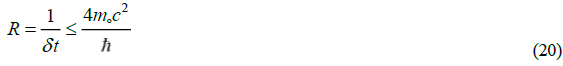
At any time our field has a 50% chance of encountering a pair and compounding that a 50% chance of annihilating and passing the baton to the newly minted field. This equal weighting can be explicitly derived, see chapter 3 in [22]. So in total it has a 25% chance of being replaced. This rate turns into an equality since the only virtual field pairs that can interact with original field must have the identical energy as these are conservative processes. This rate of replacement is 1/4 the rate of pair production.
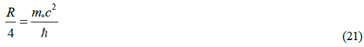
The inverse of the rate R / 4 is a mean interval any particular field lives and the distance light can travel in that interval is which now can be computed from equation. 21.
This is the Compton relation produced from a real disorder parameter, ∈. The net effect on our field is set by the mean rate of exchanging fields and generating a locality for a particle with inertia as its local position is unknown to a mean random value∈. The angular coordinate description is lost in the self-reference frame as it is reset to the present position of the particle’s center of symmetry. By randomizing the local location of the fields center of symmetry a particle is created with a finite scale along with local isotropy. The origin of the field always has to keep shifting after each annihilation to the replacement field’s partner. This randomannihilation walk generates a location, a fuzzy location, but a location that can be described. The coordinates in time and space are now statistically independent of the original laboratory frame from where they were created. So from the laboratory frame with the physical property that allows pair-production for short intervals a localized entity can be created from something very rare, an absolutely fair game of chance. This game of chance generates a statistically isolated space independent of the laboratory frame with the particle’s instantaneous frame of reference tied to the current field.
Massless fields in self-reference frame
To generate a massless field in the self-reference frame there are two choices, either set the mass to zero or make it complex. There is no choice in the laboratory frame where the mass is zero for a massless field. In the self-reference frame setting the mass to zero will not yield a state equation for the field. However, making the mass complex in the self-reference frame will generate physical field solutions and quantize the fields. This question has a long history that has produced a number of theories, however, not until the self-reference frame was found did this transformation make sense [23].
Mass is inversely related to the random variable to make mass complex must be made complex. By making ∈ complex it is equivalent to introducing a phase shift and this should be retarded so the transformation that will be used is found in equation 23 because ∈> 0 for generating a real mass. This random displacement is always positive in a spherical coordinate system as it is referenced from the instantaneous center of symmetry that is changing. Therefore for the complex displacement the relation in equation 23 is used.

To transform the remaining parameters into field equations to test the conjecture about a complex mass, it is first necessary to understand how γ in the self-reference frame transforms.
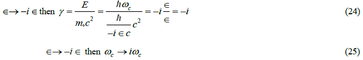
For the case in the self-reference frame when the Compton wave length is set equal to the random displacement parameter, -i∈, then γ → -i . This is one of the more important relationships derived, because it essentially enforces the quantized condition on the resultant field. In particular this is also the quantum condition for the photon energy.
A particle in the self-reference frame to participate in an electromagnetic transition or the exchange of energy with an electrostatic field must be able to changeγ . For a massless field either boson or fermion it is necessary that γ is a fixed complex constant that cannot vary. Therefore, the field either exists or doesn’t exist with no decay mechanism. The constraint that γ = -i confirms the original conjectures by Planck and Einstein that radiation is quantized. This is not the mechanism of energy exchange for an electrostatic interaction only for a radiative transition for a real photon.
The self-reference frame places a strict conditions on the material parameters that are defined in this independent space. If the
equivalent complex random displacement is applied to the particle description  The massless field’s
differential equations become:
The massless field’s
differential equations become:
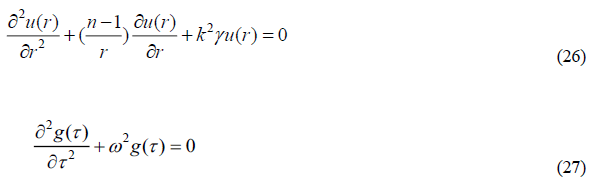
The solutions in three dimensions are:
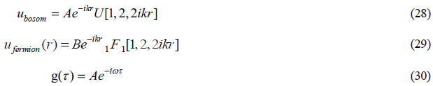
The complete solutions are then:
Now that both elementary particle and field structures have been derived their density functions in three dimensions are plotted in FIG. 1. The total wave function in the self-reference frame 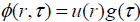 the time dependence being of the form
i e-iωτ becomes
a constant factor in the probability density function. The particle density in the self-reference frame in three dimensions is given by
the expression
the time dependence being of the form
i e-iωτ becomes
a constant factor in the probability density function. The particle density in the self-reference frame in three dimensions is given by
the expression  The core of density
  in the case of a massive fermion is proportional to the static electric field
and removes the singularity of the point electron at its center of symmetry [22]. In the case of the massive boson the properties of
weak charge result and the description is found in [23]. For the massless fields the boson density is a constant as it is for the photon
field. However, for the fermion field it has a spatial oscillatory behavior that will affect a number of properties. It is the energy
dependent oscillatory character of the density function that is of primary interest as it reduces the particles interaction cross section.
in the case of a massive fermion is proportional to the static electric field
and removes the singularity of the point electron at its center of symmetry [22]. In the case of the massive boson the properties of
weak charge result and the description is found in [23]. For the massless fields the boson density is a constant as it is for the photon
field. However, for the fermion field it has a spatial oscillatory behavior that will affect a number of properties. It is the energy
dependent oscillatory character of the density function that is of primary interest as it reduces the particles interaction cross section.
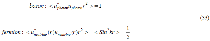
The mean value of the Sin2 term is exactly one half. This behavior in the spatial portion of the wave function is unique among particles and will lead to a reduction in detected sensitivity by exactly 50% in measured data whether from solar or reactor generated electron neutrinos.
The extensive literature on the neutrino-cross section as a function of energy that result are dynamic calculations at a level above of the density calculation for the neutrino in the self-reference frame [13]. The kinematic models do not involve the structure of the particles themselves, only their bulk properties and allowed interactions. It is not necessary to involve the specific mechanisms for the energy dependent calculation of cross-sections, because the correction being introduced will affect the neutrino across its entire energy range uniformly.
In three dimensions the complex mass generates two massless fields that appear to have real physical counter parts: photon and the electron neutrino. First is a boson with a unit density characteristic of a basic photon and then a massless elementary fermion representing a neutrino. These are solutions in the self-reference frame and not in the laboratory frame where their complete structure is developed. Both solutions are of massless fields showing no preferred local structure, see FIG. 1. This was forced by γ = -i being fixed complex constant. Any other values of γ = -i produced divergent solutions that are not valid. Divergence here means that the density functions grow larger with increasing r , which is neither the property of a physical realizable particle or field. Fixing γ for massless field also insures the independence of the speed of light in any reference frame. This restriction on γ is a requirement for the quantization of the field for both the photon and neutrino.

Figure 1: Density functions of fields and particles in the self-reference frame. The individual density scales are arbitrary so the functions separate. The parity problem of the massive bosons can be seen at r=0 as the density function in its dependence on γ and is independent of γ for fermions [22].
In the self-reference frame the harmonic time dependence of a stable entity that starts with a private time dependence when the frame is created with no previous history. All entities whether a particle or a field come with their own clocks, via their time dependence, and are essentially isolated by the statistical independence of the space in which they were generated. The only exception is when two or more particles share the same clock either from being created at the same instance or interacting with one of two fields or particles that were created as a pair. This behavior of particles and fields sharing a self-reference frame is important for understanding entanglement.
The original requirement for special relativity as laid out by Einstein 1905 are the existence of a measurement scale and a time base. Both conditions are satisfied for each individual particle and quantized field by their properties in their self-reference frame. No external observer is required to fulfill these needs for a clock and a ruler.
Massless fields in the laboratory frame
Taking equation 34 and setting mass to zero yields the wave equation for massless fields with an interaction term that generates the refractive index when the fields encounter matter.
This makes a more general coupling between quantum mechanics and electromagnetic theory as quantum mechanics generates the propagating field behavior that is found in the Faraday-Maxwell theory. This equation is equally valid for any massless propagating field such as the neutrino. Now refraction for both the photon and neutrino can be treated as a potential interaction with a physical medium.
Borexino Data
The ve detection method is to monitor the scattering process (ve , e-) in a large liquid scintillator [24]. The Borexino analysis assumes the standard solar model chain of coupled fusion reaction and decays generates a distribution of isotopes that is accurate from an end point analysis of star surface chemistry. To do this analysis one has to assume that knowledge of all possible reactions are included and accurately accounted for including the dependence on the distribution of material throughout the sun as a function of depth and temperature. The second assumption is that the calculated kinetic neutrino cross section is assumed to be correct, because there is a good understanding of the weak processes. The strength of the analysis and experiment is that most of the activity with the ve occurs for processes that can be individually isolated. The data of interested is presented in TABLE 2.
If the neutrino density function from equation 33 is correct there will be a factor multiplying the flux measurements which is 0.5 and
the average of the unweighted five process is  This unweighted result is very close to the expected decrease computed
for the reduction produced by the neutrino density function. Because of the manner of experimentally isolating individual components
the best comparison that can be made is an unweighted mean. Tying the deficit of neutrinos to a reduction in neutrino flux rather than
a reduction in detector sensitivity across a significant energy range leads to a false conclusion about e v mass. The data indicates the
solar e v is a stable massless field (TABLE 1).
This unweighted result is very close to the expected decrease computed
for the reduction produced by the neutrino density function. Because of the manner of experimentally isolating individual components
the best comparison that can be made is an unweighted mean. Tying the deficit of neutrinos to a reduction in neutrino flux rather than
a reduction in detector sensitivity across a significant energy range leads to a false conclusion about e v mass. The data indicates the
solar e v is a stable massless field (TABLE 1).
TABLE 1. Probability of solar neutrino survival data from Borexino [24]. The pp and the 7Be have continuous neutrino
spectra down to zero energy. The pp process is the dominant process but with a small detection cross-section making it
more difficult to resolve at low energy. The mean on the unweighted sum of the survival probability is 
| Energy (MeV) | Process | Mean | Low | High |
|---|---|---|---|---|
| 0.3-0.4 | 1H +1H →2H + e+ + νe | 0.64 | 0.52 | 0.76 |
| 0.89 | 1H + 1H + e− → 2H + ν | 0.62 | 0.47 | 0.79 |
| 1.5 | 7Be + e− → 7Li + ν | 0.52 | 0.46 | 0.58 |
| 3-18 | 8B + e− → 8Li + νe | 0.38 | 0.27 | 0.51 |
| 5-18 | 8B → 8Li + e+ + νe | 0.31 | 0.22 | 0.43 |
| 0.3-18 | Means (theory 0.5) | 0.494 | 0.388 | 0.614 |
Discussion
After WWII quantum field theory adopted complex perturbation theories, gauge particles, symmetry arguments, along with higher dimensional spaces as a basis for quantum field theories ensuring no progress would be made [2]. Complex symmetries and duals are end points not a starting point in describing the basis of matter. The principal tool used by these modelers was the Hilbert vector space to encapsulate unknown properties that would be sorted out at a later date. The assumption of this vector space inhibited any inspection of the real physical spaces it was supposed to describe. In effect both the particle/field private spaces were mashed together with dynamical space of the laboratory frame. This produced a mess that was difficult to untangle and thwarting the analysis produced by J.S. Bell and others to unravel the problem. Models evolved for high energy and low energy processes that were entirely disconnected, where there should have been a common analysis (TABLE 2).
TABLE 2. Main predictions from quantum mechanics using a relativistic basis from 2014 to the present.
| Prediction |
| Measurement Problem removed with coupled spaces [12] |
| Two particle families: Bosons and Fermions [12] |
| Force field basis of particle structure Quantized fermion charge [12, 14] |
| CP violation for massive 3D boson [12] |
| Basis for superposition [22] |
| Basis for Pauli Principle [16] |
| Hydrogen 2S and 2P no longer degenerate [14] |
The strong influence of classical energy handling in thermodynamics, mechanics, along with Hamilton’s principle weighed on the thinking of Einstein, Dirac, and those that followed freezing quantum mechanics into a form that had developed by the late 1920s [2, 3]. The people that followed Dirac spawned numerous models for physics and cosmology using the methods he introduced. His delta function was used to tame the singularity of the point particle and his sea of positrons produced a very complex vacuum. By 1932 it was too late to change course as a school had been built up in northern Europe that appealed to the minds of theorist who copied the license Dirac originally claimed to create models independent of empirical data.
The combination of lower dimensional components to construct baryons and meson looks promising [22]. While the mathematics of these spaces not dependent on the mathematical continuum will change the tools used. As quantum mechanics needed to properly account for relativity, so did special relativity need to deal with the bound state and antiparticles.
Acknowledgments
First to Jack Steinberger who in an elementary physics course to a group of freshmen in 1966 stated he had forgotten classical mechanics and it was only possible for him to teach quantum mechanics. This made perfect sense as quantum mechanics cannot be derived from classical mechanics. After introducing the Schrödinger equation a student named Peter Landesman asked “What would be the result if mass in the Schrödinger would be a complex number?” Attempts to answer this question has unduly complicated physics. Then he introduced an additional problem with quantum mechanics in the question about how primitive longitudinal fields in physics are poorly understood. Secondly to Polykarp Kusch whose experimental efforts to show quantum electrodynamics was built on a false foundation proved correct.
Recently we are grateful to Glenn Westphal for his discussion on the Copenhagen view of quantum mechanics and Doug Higinbotham who explained the nuclear short range correlation data and the schemes used to model high energy electron scattering. Finally to Fabbio Mazzolai and Ganapati Myneni both impatient with the hydrogen-in-metals community triggered a reexamination of the effects hydrogen contamination in superconducting accelerator cavities that led to a result of how mass can be defined from studying the limits of quantum diffusion in metals.
References
- Formaggio JA, Zeller GP. From eV to EeV: Neutrino cross sections across energy scales. Rev. Mod. Phys. 2012 24;84(3):1307.
- Gamow G. Thirty years that shook physics: The story of quantum theory. Anchor Book, NYC 1966
[Google Scholar][Crossref]
- Halpern P. Einstein's Dice and Schr dinger's Cat: How Two Great Minds Battled Quantum Randomness to Create a Unified Theory Phys., Basic Books; 2015 14.
[Google Scholar][Crossref]
- Kac M. Random walk and the theory of Brownian motion. Am. Math. Mon.1947;54(7P1):369-91.
- Kac M. On distributions of certain Wiener functionals. Trans. Am. Math. Soc. 1949;65(1):1-3.
[Google Scholar] [Crossref]
- Kac M, Carus mathematical monographs n. 12. Statistical Independence in Probability. Maa; 1959 Mar.
[Google Scholar] [Crossref]
- Kac M. Can one hear the shape of a drum?. am. math. mon. 1966;73(4P2):1-23.
- Dodd CV, Deeds WE. Analytical solutions to eddy‐current probe‐coil problems. J. appl. phys. 1968;39(6):2829-38.
- Wallace, J. SSTIN10 AIP Conference Proceedings 1352, edited by G. Myneni and et. al. (AIP, Melville, NY) 2011:205-312.
[Google Scholar] [Crossref]
- Wallace JP. Electrodynamics in iron and steel. arXiv preprint arXiv:0901.1631. 2009.
- Wallace JP. Spintronics enter the iron age. JOM. 2009;61(6):67-71.
[Google Scholar][Crossref]
- Wallace JP and Wallace MJ. The Principles of Matter: Amending Quantum Mechanics. Cast. Anal. Corp.; 2014.
[Google Scholar][Crossref]
- Formaggio JA, Zeller GP. From eV to EeV: Neutrino cross sections across energy scales. Rev. Mod. Phys. 2012 24;84(3):1307.
- Wallace JP and Wallace MJ. Electrostatics. In AIP Conference Proceedings. AIP Publ. LLC 2015;1687(1):040004. [Google Scholar][Crossref]
- Slater L. J.Handbook of Mathematical Functions with Formulas, Graphs, and Mathematical Tables, ASM 55, edited by M. Abramowitz and I. Stegun (Dept. of Commerce, Washington DC) 1968:503-36.[Google Scholar] [Crossref]
- Wallace JP, Wallace MJ. “The bound state” vixra:2103.0026.2021[Google Scholar] [Crossref]
- Wallace JP, Wallace MJ. Nuclear Structure and Cold Fusion. J. OF CONDENS. MATTER NUCL. SCI. 2020.
[Google Scholar][Crossref]
- Dirac PA. Relativistic quantum mechanics. Proceedings of the Royal Society of London. Series A, Containing Papers of a Mathematical and Physical Character. 1932;136(829):453-64.
- Pauli W, Weisskopf VF. Über die Quantisierung der skalaren relativistischen Wellengleichung. Wolfgang Pauli: Gewissen Phys. 1988:407-30.
[Google Scholar][Crossref]
- Dirac PA. The principles of quantum mechanics, 4th edn. Clarendon. 1958
- Bethe HA and Salpeter EE. Quantum mechanics of one-and two-electron atoms. Springer Sci. Bus. Media; 2012(6).
[Google Scholar][Crossref]
- Wallace J and Wallace M. “yes Virginia, Quantum Mechanics can be Understood”. Cast. Anal. Corp., Weyers Cave, VA. 2017.
[Google Scholar][Crossref]
- Feinberg G. Possibility of faster-than-light particles. Phys. Rev. 1967;159(5):1089.
- Derbin A, Muratova V, Agostini M, at al. The Main Results of the Borexino Experiment.1605.06795. 2016 (22).