Research
, Volume: 11( 5) DOI: 10.37532/2320-6756.2023.11(5).341From black-body radiation to gravity: why neutrinos are left-handed an why the vacuum is not empty
- *Correspondence:
- Engel Roza Philips Research Labs, Eindhoven, The Netherlands, E-mail: engel.roza@onsbrabantnet.nl
Received date: 01-May-2023, Manuscript No. tspa-23-97503; Editor assigned: 03-May-2023, PreQC No. tspa-23-97503 (PQ); Reviewed: 06May-2023, QC No. tspa-23-97503 (Q); Revised: 08-May-2023, Manuscript No. tspa-23-97503 (R); Published: 15-May-2023, DOI. 10.37532/2320-6756.2023.11(5).341
Citation: Roza E. From Black-Body Radiation to Gravity: Why Neutrinos Are Left-Handed and Why the Vacuum Is Not Empty. J. Phys. Astron.2023;11(5):341.
Abstract
Starting from an overview of neutrino problems and a simplified survey of Fermi’s neutrino theory, it is shown why neutrinos are lefthanded and why they seem to show an oscillatory behaviour between their flavours. After addressing the question of how to assess the naked mass of the true elementary particles, it is hypothesized that the elementary constituents of the nuclear background energy and the cosmological background energy are the same. This allows us to derive the magnitude of the quark’s “naked” mass from the polarization of the vacuum.
Keywords
Neutrino; Fermi constant; Parity violation; Dark matter
Introduction
In the history of the development of the theory for particle physics described so far, the description of three dilemmas that have preeminently been decisive for the current Standard Model has been omitted still [1]. These dilemmas have to do with the neutrino, which so far in this review has been barely mentioned. The history of the neutrino begins with a misunderstood phenomenon from the years before 1930.
First surprise
One would expect in radioactivity, in which nuclear particles change state, that the energy difference between the particle that has not yet decayed and the decayed particle is carried away by particles with a discrete energy value. This was the case with alpha radiation carried by nuclei of the Helium atom. Curiously, it was not the case with beta radiation carried by electrons. The spectrum of the electron beam turned out to be continuous rather than discrete like illustrated in FIG. 1. That was already apparent in 1914 from observations by James Chadwick (who became famous in 1930 for the discovery of the neutron) and others. It was a problem that led Wolfgang Pauli in 1927 to formulate a bold hypothesis which he did not dare to publish, but sighing posited in a letter to Hans Geiger and Lise Meitner [2]. Because, unlike some other scientists, including Niels Bohr, he did not want to doubt the law of energy conservation, he suggested in the letter the existence of a particle that eludes observation. That particle should be nearly massless, electrically neutral, and have a half-integer spin. He called that particle "neutron", a name that was changed to neutrino after Chadwick discovered the neutron. It was Enrico Fermi who took Pauli's hypothesis seriously and in 1933 developed a theory for beta radiation based on the neutrino existence [3]. Incidentally, the existence of the neutrino was not experimentally confirmed until 1956 by Reines and Cowan [4].

Figure 1: Expected density spectrum of the electron’s energy in beta radiation (red) and the observed one (black).
Second surprise
The decay process in radioactivity turned out to have a second surprise. One would expect that the spin of the electrons in the beta radiation does not favour a polarization direction. After all, there is no immediate plausible physical explanation why electrons in the beta radiation would in this respect not be on par. About 1956, Tsung-Dao Lee and Chen-Ning Yang began to doubt this based on observations of the decay process of the kaon meson. In a scientific review, they concluded that the parity of the weak interaction should be questioned [5]. Shortly afterwards, they approached Chen-Siung Wu with the question of whether she could provide an experimental answer. Much to the surprise of many, she succeeded [6]. She did so by analyzing the beta radiation released by the radioactivity of the Cobalt-60 atom and found that the electrons in the beta radiation have a left-handed spin. Afterwards, it could be established that this phenomenon occurs in all other decay processes determined by beta radiation. The weak interaction, therefore, turned out to be a force that, unlike the electromagnetic or the strong interaction, violates the parity of natural forces. The antineutrino that acts as a sister particle of the electron in the decay process, is therefore right-handed and so the neutrino is left-handed. But whereas the spin of the electron can be influenced outside the decay process, there are no means to do so with the neutrino. Hence, the neutrino is always left-handed.
Third surprise
The Reines-Cowan experiment mentioned before marks the start of experimental studies on neutrinos. One of the problems, next to identifying suitable physical processes to study the interaction of neutrinos with matter, is the issue of how to obtain neutrino fluxes large and strong enough to detect the rare events expected from those processes. Reines and Rowan used a nuclear reactor for the purpose. Their experiment got follow-ups by other ionic neutrino experiments, in particular those based upon knowledge captured in the Standard Solar Model. The idea behind those is, that since the energy of the sun is known and since its major energy production mechanism as well, it is possible to calculate the neutrino flux on Earth as well. This flux is defined as the number of neutrinos that, each second pass through a 1m square surface perpendicular to the direction of the sun. This would enable to development experimental evidence not only in qualitative terms but in quantitative terms as well.
And it did. Most remarkably, however, in 1976 those experiments revealed an unexpected result [7]. The predicted neutrino count showed a deficit of about 50%-70% concerning the measured count. The solar neutrino problem was born. What happened with the neutrinos emitted by the sun? Why would those not be capable to produce the predicted neutrino count? The inevitable answer to the problem is the awareness that neutrinos are subject to changes when they move from the sun to the detectors on Earth. The simplest approach to this problem is the assumption that neutrinos come in different flavors. Because they are produced in co-production with charged leptons, they show a specific flavor determined by the co-produced charged lepton. This hypothesis could be affirmatively tested by making the neutrino detectors in the experimental equipment no longer exclusively sensitive to electron neutrinos. Nevertheless, a major problem remained: the neutrino flow from the sun is produced from the nuclear fusion of Hydrogen atoms into Helium nuclei, thereby producing almost exclusively electron neutrinos. How to explain the change of electron neutrinos into a significant amount of other flavors on their route from the sun to Earth?.
Eventually, this tantalizing question has resulted in accepting a bold hypothesis, earlier formulated by Pontecorvo in 1957, and later adopted as an explanation for the missing neutrinos, that neutrinos are built up by a virtual substructure [8]. Such a virtual substructure would allow neutrino compositions built by three basic eigenstates, different from their flavor states, more or less in the same way as hadrons are composed by quarks. According to this hypothesis, the electron neutrino is in a particular mixture of eigenstates, while a muon neutrino and a tauon neutrino would be in other mixtures. Hypothetically, this would allow oscillations between the flavour states of neutrinos and the loss of coherency would solve the solar neutrino problem. If substructures are considered as being viable for neutrinos, why would substructures for charged leptons not be viable as well? Why not conceive the electron, the muon and the tauon as states built by underlying constituents as well? Within the Standard Model, the charged leptons are simply considered as elementary particles, and because, in the Standard Model, everything comes in a three, even a basic question such as “why no charged lepton beyond the tauon” has remained unanswered. In recent work, I have shown how these issues of the constrained lepton generation and the mass and origin of neutrinos can be highlighted in the structure-based model of particle physics, documented in [1,9].
Around the mid-1970s, when the Standard Model of particle physics has been conceived, the massless property and the left-handiness of neutrinos has been taken for granted. Although the descriptive nature of the Standard Model does not require so, it would have been more satisfying if some physical understanding could be found that would justify the acceptance of the zero mass and the lefthandiness axioms. The more, because experiments on neutrinos presently give reasons to put the mass-less property of neutrinos into doubt. It is probably fair to state that the present state of the Standard Model does not give the proper picture of the neutrinos. The theory captured in the Standard Model is not capable to describe the oscillatory phenomenon between flavour states. In 1962 this oscillatory phenomenon has been heuristically captured in the PMNS matrix (Pontecorvo, Maki, Nakagawa, Sakata) description of a neutrino [10]. It is based upon a flavour decomposition in a flavour-dependent mix of eigenstates. Description, however, is not the same as understanding. In the recent work just mentioned it has been shown how a structure-based analysis of the pion’s decay path explains the origin and the properties of these eigenstates [9]. An explanation of why neutrinos are left-handed, though, is still missing. The structural model as discussed in the first part of this essay [1] is a useful starting point to highlight the three issues mentioned in this introduction in more detail. The next paragraph contains a summary of that model.
Structural Models for Pion, Muon and Neutrino
FIG. 2 is an illustration of the structural model for a pion as developed by the author over the years [1]. It shows that two quarks are structured by a balance of two nuclear forces and two sets of dipoles. The two quarks are described as Dirac particles with two real dipole moments as the virtue of particular gamma matrices. The vertical one is the equivalent of the magnetic dipole moment of an electron. The (real-valued) horizontal dipole moment is the equivalent of the (imaginary-valued) electric dipole moment of an electron [11,12].
In a later description, after recognizing that this structure shows properties that match with a Maxwellian description, the quarks have been described as magnetic monopoles in Comay’s Regular Charge Monopole Theory (RCMT), [13,14]. This allows us to explain the quark’s electric charge by assuming that the quark's second dipole moments (the horizontal ones) coincide with the magnetic dipole moments of electric kernels. This description allows us to conceive the nuclear force as the cradle of baryonic mass (the ground state energy of the created anharmonic oscillator) as well as the cradle of electric charge.

Figure 2: Hypothetical equivalence of the quark’s polarisable linear dipole moment with the magnetic dipole moment of its electric charge attribute.
The model allows a pretty accurate calculation of the mass spectrum of mesons. It also allows the development of a structural model of baryons including an accurate calculation of the mass spectrum of baryons as well. This calculation relies upon the recognition that the structure can be modelled as a quantum mechanical anharmonic oscillator. Such anharmonic oscillators are subject to excitation, thereby producing heavier hadrons with larger (constituent) masses of their constituent quarks. The increase of baryonic energy under excitation is accompanied by a loss of binding energy between the quarks. This sets a limit to the maximum constituent mass value of the quarks. It is the reason why quarks heavier than the bottom quark cannot exist and why the top quark has to be interpreted differently from being the isospin sister of the bottom quark [1].
Because lepton generations beyond the tauon have not been found, they probably don’t exist for the same reason. In such a picture the charge lepton structure would result from the decay loss of the magnetic charges of the kernels in the pion structure under simultaneous replacement by their electric charges. This structure is bound together by an equilibrium of the repelling force between the electric kernels and the attraction force between the scalar dipole moments. Despite its resemblance with the pion structure, its properties are fundamentally different. Whereas the pion consists of a particle and an antiparticle making a boson, the charged lepton consists of two kernels making a fermion. FIG. 3 shows a naive picture of the decay process. Under decay, the pion will be split up into a muon and a neutrino. In the rest frame of the muon, the muon will contain the electric kernels and some physical mass. The remaining energy will fly away as a neutrino with kinetic energy and some remaining physical mass. FIG. 3 shows the model, in which a structure less neutrino is shown next to a muon with a hypothetical substructure.
In this picture, the muon is considered to be a half-spin fermion despite the appearance of two identical kernels in the same structure. Assigning the fermion state to the structure seems to conflict with the convention to distinguish the boson state from the fermion state by a naive spin count. Instead, a true boson state for particles in conjunction should be based on the state of the temporal part of the composite wave function. In this particular case, the reversal of the particle state into the antiparticle of one of the quarks marks a transformation from the bosonic pion state into the fermionic muon state under the conservation of the weak interaction bond.
Let us proceed from the observation that there is no compelling reason why the weak interaction mechanism between a particle and an antiparticle kernel would not hold for two sub-particle kernels. In such a model, the structure for the charged lepton is similar to the pion one. It can therefore be described by a similar analytical model. Hence, conceiving the muon as a structure in which a kernel couples to the field of another kernel with the generic quantum mechanical coupling factor, the muon can be modelled as a one-body equivalent of a two-body oscillator, described by the equation for its wave function Ψ,

Figure 3: The decay of the pion’s atypical dual dipole moment configuration into two typical single dipole moment configurations.
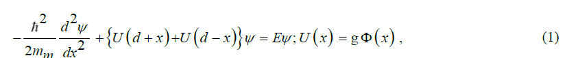
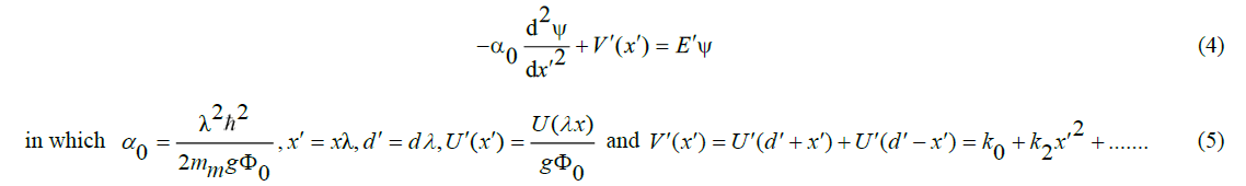
Which h is Planck’s reduced constant, 2d the kernel spacing, mmthe effective mass of the centre, V(x)=U(d+x)U(d-x) its potential energy, and E the generic energy constant, which is subject to quantization. The potential energy V(x)an be derived from a potential  . Similarly, as in the case of the pion quarks, this potential is a measure of the energetic properties of the kernels. It is characterized by strength
  (in units of energy) and range
  (in units of length: the dimension of is [m-1]).
The potential of a pion quark has been determined as [1],

These quantities have more than symbolic meaning, because the structural model for particle physics developed so far [1], λ has been quantified  in which
  is the energy of the Higgs particle as the carrier of the energetic background field. The quantity has been quantified by
  , in which
  is the energy of the weak interaction boson. An equal expression for the potential ()xwould make the muon model into a Chinese copy of the pion model.
Instead, we wish to describe the potential ()xof the muon kernels as,
The rationale for this modification is twofold. In the structural model for the pion, the exponential decay is due to the shielding effect of an energetic background field. If the muon is a true electromagnetic particle, there is no reason why its potential field would be shielded. This may explain why an additional energetic particle (the neutrino) is required to compensate for the difference between the shielded and the unshielded potential. As shown in the Appendix of ref., the format of the wave function holds along the dipole moment axis of two-body structures with energetic monopole sources that spread a radial potential field 1/r and a dipole moment field  along the dipole axis [9].
imilarly, as in the pion case, it will make sense to normalize the wave function equation too,
In which and are dimensionless coefficients that depend on the spacing 2 between the quarks. To proceed, it is imperative to establish a numerical value for the constant. This touches on an essential element of the theory as outlined in this essay. In a classical field theory, the baryonic mass has no relation with the potential field parameters in terms of strength, range and coupling constant. In this case, however, the bare mass of the two kernels doesn’t contribute to the baryonic energy built up in the anharmonic oscillator that they compose. This baryonic energy distributed over the two kernels can be conceived as a constituent mass that composes. In previous work [15,16] it has been shown that Einstein’s theory of General Relativity (GR) allows us to calculate this baryonic energy from the potential field of the two kernels. This requires the recognition that the kernels are Dirac particles with particular gamma matrices giving the kernels a real-valued second dipole moment, thereby giving rise to a quasi-harmonic nature to the quantum mechanical oscillator that they build.
This view enables us to identify as [1,15,16],
I wish to emphasize that these two elements, i.e. application of Einstein’s GR and recognition of the particular nature of the quarks as Dirac particles of a particular type, have not been recognized, hence not been credited), in the Standard Model of particle physics. It makes a structured model as outlined in this essay possible, thereby revealing quite some unrecognized relationships between quantities and concepts that in the present state of particle physics theory are taken as axioms.
The muon model shown by (4) and (5) is the same as the model of the pion discussed in [1]. The potential function of the kernels, though, shown in (3) is slightly different. This has an impact on the constants, but that is all. It means that similarly to the pion meson, charged lepton muon is subject to excitation. It explains why the tauon can be conceived as a scaled muon. The muon and the tauon are charged leptons in different eigenstates. The kernel spacing in the tauon is smaller than in the muon, thereby increasing its rest mass. Details can be found in [9]. FIG. 4 shows the result. The calculated tau mass is 1.89 GeV/c2. This is rather close to the tau particle’s PDG (Particle Data Group) rest mass (1.78 GeV/c2), [17]. The difference is due to a slight inaccuracy in the calculation. The picture shows that the loss of binding energy prevents the existence of other charged leptons.
The pion model shown in FIG. 2 illustrates that the polarity of the real-valued second dipole moments of the quarks is fixed by the structure. It implies that the polarity of the magnetic dipole moments of the two electric kernels is fixed by the structure as well. This loss of freedom in the orientation of the dipole moments is the reason why the initial spatial orientation of the dipole moment of a muon that results from the pion decay is not a free choice. Once made free, the dipole moment orientation (= spin) of the muon can be influenced by external influence. This, however, cannot be done for the accompanying neutrino in the decay process, because of its insensitivity to external influences. It explains why neutrinos are left-handed.

Figure 4: The lower curve shows the dependence of the lepton’s physical mass on the pole spacing. The upper graph shows that the pole spacing of the tau particle is determined by the equality in vibration energy of the muon’s first excitation level and the ground state vibration energy of the heavier tau particle. Note that the binding energy of the tau particle is just slightly negative
Fermi’s Theory
Unfortunately, the excitation model muon-tauon does not hold for the electron-muon relationship. Whereas the muon and the tauon are interrelated because of their internal weak interaction bond, such a bond does not exist for the electron, because the electron is produced as a decay from the muon caused by the loss of this bond. It is instructive to analyze this decay process based on Fermi’s theory, which as a forerunner of the weak interaction theory by Wbosons, describes the origin of the neutrinos as the inevitable consequence of the shape of the energy spectrum of electrons shown in measurements on beta decay.
Fermi's model is conceptually simple, but rather complex in its implementation. For this essay, a simplified representation will suffice, illustrated in the left-hand part of FIG. 5.

Figure 5: Fermi’s beta decay model with direct coupling versus decay by weak interaction boson.
This shows the decay of a neutron into a proton under, the release of an electron. To satisfy the conservation of energy, the energy difference between E0 the neutron and the proton must be absorbed by the energy Eof the electron and the energy pvcof the neutrino moving at about the speed of light. To satisfy momentum conservation, the momentum Pof the nucleon must be taken over by the momenta peand pv of the electron and neutrino, respectively, so that

To explain the occurring energy spectrum of the electron, Fermi has developed the concept of density of states. This is based on the assumption that fermions, such as the electron and the neutrino, despite their point like character, require a certain spatial space for their wave function that does not allow a second wave function of a similar particle in the same space. That comes down to respecting the exclusion principle that was posited by Pauli in 1925 in the further development of Niels Bohr's atomic theory from 1913.
In a simple way, that spatial space is a small cube whose sides are determined by half the wavelength (/2L) of the fermion. A volume Vcontains N fermions. So,

For a particle in a relativistic state holdspc hω=pc. In that case, after differentiating,
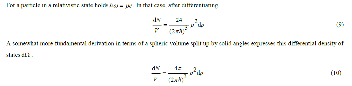
The difference is about a factor of 2. The difference can be explained because the roughly derived quantity admits two particles in the interval by taking into account a difference in spin. The differential density of states that can be attributed to the decay product of neutron to proton is equal to the product of the contributions of the electron and of the neutrino, so that,
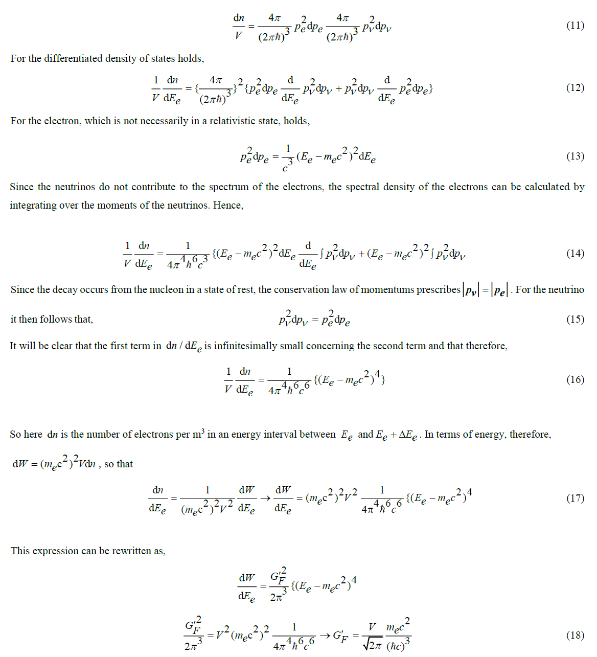
The relationship takes on a simple form if the decay product is relativistic. This is usually true when muons decay into electrons, because in the major part of the spectrum E>>mec2.In that case,
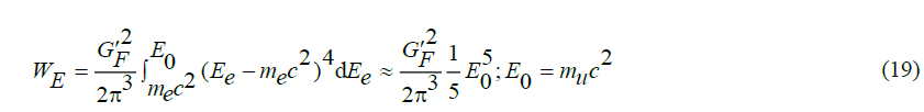
The relevance of this expression becomes clear from Fermi's "Golden Rule", which relates the half-life τ (in which half of a nuclear particle decays) and the integral WE of the decay spectrum,
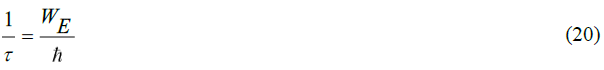
This expression shows that the lifetime of a nuclear particle is determined by the time it takes to build up the decay spectrum with the total energy valueWE. Note that the expression resembles Heisenberg's uncertainty relation,

The rule is based on a statistical analysis of the decay process, the details of which can be found in the literature [18, 19]. The calculated energy density spectrum is shown in FIG. 6. The fifth-power shape, which relates the massive energy mc2 of a nuclear particle to its decay half-life, is known as (Bernice Weldon) Sargent's law, as formulated empirically in 1933.
It would be nice if it would appear to be possible to derive by theory an estimate for the numerical value of GF. Let us see if this can be done.
If we would know V, the constant GF can be calculated. Since the calculation of the density of states assumes the spatial boundary of the wave function of the decay products, it is reasonable to assume that the volumeVis determined by the spatial boundary of the wave function that fits the energy from which the decay products originate, so that

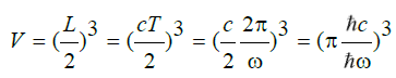 , and therefore
in which hωnp the energy determines the formation of the decay products. As illustrated in the right-hand part of FIG. 5, Fermi’s point contact model has been revised after the discovery of Wbosons as carriers of the weak force, which is seen as the cause of the decay process. This insight led to the model shown in the right half. Zooming in on it shows that neutron decay is caused by the change in the composition of the nucleon 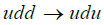 . This is shown in the left-hand part of FIG. 7. This picture is symbolic because it suggests that the energy difference between a uquark and a dquark is determined by a Wboson, while we know that the free state energy of a boson is 80.4 GeV and there is only a 1.29 MeV mass difference between the (udd) neutron and the (udu) proton.
The figure in the middle gives a more realistic picture of the Wboson. A positive pion decays in its entirety via a Wboson into a (positive) muon and a neutrino. It is more realistic because earlier in this essay we established that the pion moving at about the speed of light has a rest mass of 140 MeV, while it behaves relativisticly as 80.4 GeV before its decay into the muon's rest mass of 105 MeV plus neutrino energy (that in the rest frame of the muon corresponds to a value of about 39.5 MeV). A (negative) muon in turn decays into electrons and antineutrons as shown in the right part of the figure. It will be clear from these figures that one W boson is not the other. Only the middle image of FIG. 7 justifies its energetic picture. Hence, as discussed earlier in the essay, the 140 MeV rest mass of the pion is the non-relativistic equivalent of the 80.4 GeV value of the boson.

Figure 7: tspa-11-5-97503-g007
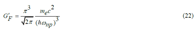
These considerations lead us to consider the decay process from pion to muon to be the most suitable one to calculate the constant GF . Because the pion decays to a muon, the rest mass of the muon (= 100 MeV) takes the place of the electron before. The energy hωnp from which the decay product arises is the energy of the free state Wboson, so that
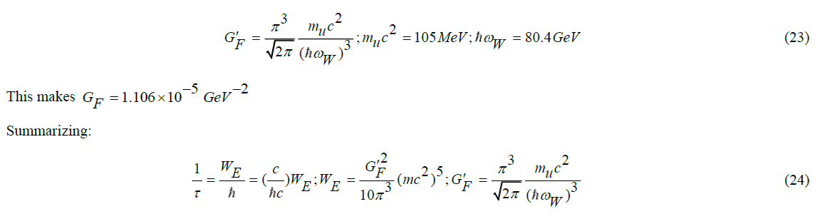
Let us emphasize that in this text the result is obtained by theory. The canonical theory is less predictive. Instead, the empirically established value of the muon’s half-life is invoked for giving an accurate value for Fermi’s constant. The analytical model described in Griffith's book gives as canonically defined result [9]. This result has a predictive value because it allows us to calculate the decay time of any nuclear radioactive particle from the reference values of, respectively, the weak interaction boson ( hωW =80.4GeV ) and the massive energy of the muon  The result thus calculated for the muon itself is
  This compares rather well with the experimentally established value
 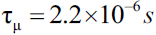 s reported by the Particle Data Group (PDG) [17]. Let us emphasize that in this text the result is obtained by theory. The canonical theory is less predictive. Instead, the empirically established value of the muon’s half-life is invoked for giving an accurate value for Fermi’s constant. The analytical model described in Griffith's book [19]. It gives a canonically defined result,
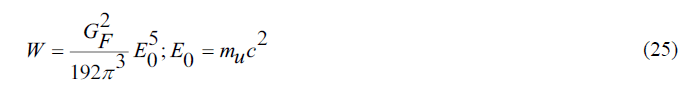
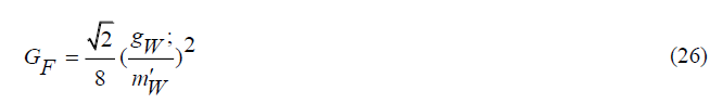
The factor 192 (= 2 × 8 ×12) is the result of integer numerical values that play a role in the analysis. Unlike the predictive model described in this paragraph, this relationship does not allow to the calculation of the decay time τμ of the muon. Instead, taking the experimentally measured result of this decay time of the muon. Instead, taking the experimentally measured result of this decay time  as a reference, the quantityGF , dubbed as Fermi’s constant is empirically established
  . It confirms the predictive merit of GF in (24).
In Griffith's book, the factorGF is deduced as,
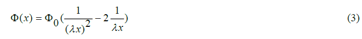
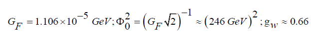
Herein gWis an unknown quantum mechanical coupling factor. In the Standard Model, this is related to the weak force boson m'W and the vacuum expectation value 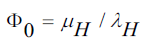 determined by the parameters of the background field, such that

This establishes a link between GF and Φ0 such that
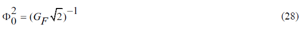
Unlike in the predictive model just described, these relations do not allow to calculation the decay time of the muon. Instead, taking the experimentally measured result of this decay time  as a reference, the quantities are numerically assigned,
For the sake of completeness it should be noted that in the weak force theory of Glashow, Salam and Weinberg (GSW), this coupling factor gW is further nuanced.
In the first part of the essay, it has been noted that the structural model, as described in the first part of this essay, has a different definition for the coupling factor and what it is based on. Whereas in the Standard Model, the coupling is defined as 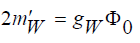 in the structural model the semantics are somewhat different. In the latter model, we have
 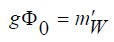 , which g is taken as the square root of the electromagnetic fine constant
 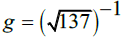 .This gives a different value Φ0.Under maintenance of the vacuum expectation relationship
 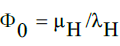 , we have different values for the Higgs parameters
 .In both models, however, we have the same semantics because of its relationship with the Higgs boson
 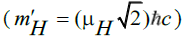 [1, 19].This makes the values and the coupling factors different, while is the same in the two cases. The solutions in three dimensions are:
The theory as described in this text does not allow us to relate the rest masses of the muon and the tauon with the rest mass of the electron. Within the Standard Model, the three charged leptons are considered elementary particles. Hence, their rest masses are taken for granted. Further detailing of the rest mass values requires a link with gravity. In this text, it has been shown that the rest mass of the muon is related by theory with the rest mass of the pion. The pion’s rest mass relies upon the rest mass of the quark. Also here, a link with gravity is needed to reveal the true value of the quark’s rest mass. It will be discussed in paragraph 5 of this article.
What can be done for the mass of the neutrino, though, is a measurement based on a careful analysis of the spectrum of beta radiation produced by the radioactivity of a suitably chosen element. FIG. 6 is suited for explaining the principle. It shows that the endpoint of the graph is characteristic of the maximum energy that an electron in the decay process may get. The difference between the measured energy of the fastest electrons with the theoretical endpoint must be equal to the rest mass of the electron neutrino. The accuracy obtained with KATRIN (KArlsruhe TRItium Neutrino) experiment, has enabled us to assess an upper limit for the mass of the electron neutrino, such that [21].
[21].
The Eigenstates of Neutrinos
Considering that the tauon is the result of the excitation of the muon modelled as an anharmonic oscillator built up by two kernels, it is worthwhile to consider the possibility that the muon neutrino is subject to excitation as well. Considering that the potential is a measure of energy and that the break-up of a pion into a muon and a neutrino takes place under the conservation of energy, it is fair to conclude that the neutrino can be described in terms of a potential function as well, such that

We may even go a step further by supposing that similarly to the muon, the neutrino can be modelled by a composition of two kernels as well. If so, each of these neutrino kernels has a potential function ΦV(x) , such that

It is instructive to emphasize that the potential function of a particle, be it a quark, a charged lepton or a neutrino, does not contain any information about its mass. In that respect, it is not different from the potential function of a charged particle like an electron. Furthermore, it is of interest to emphasize that, as mentioned before, the quantities Φ0 and λ have a physical meaning in quantitative terms. Similarly, as in the muon case, this equation can be written as,
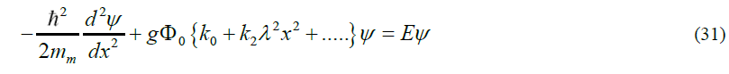
The only difference so far is that the expansion of the potential function (30) will result in other values for the dimensionless constants k0 and k2. Doing the same as with pions and muons we find three possible eigenstates before the binding energy is lost. The result is shown in FIG. 8.

Figure 8: The pole (kernel) spacing in the neutrino is determined by the equality in vibration energy of the neutrino’s first excitation level, respectively the second excitation energy from an ideal ground state with its the ground state vibration energy at reduced pole spacing. Note that the binding energy just allows three modes of eigenstates.
This eigenstate model for neutrinos shares quite some characteristics with the present adopted model of neutrinos as in 1957 heuristically proposed Pontecorvo [8]. Quite some questions, though, remain. It is for instance not clear why neutrinos should interact on their own, making different flavor states, without being influenced by their charged partners. One of the issues to be taken into consideration is the statistical character of particle physics. Taking as an example the break-down of the weak interaction of muons into electrons and neutrinos, one might expect that the produced neutrinos are not only subject to a statistical distribution of their kinetic energy but that their distribution over the three possible eigenstates is subject to a statistical behavior as well. Although in this view any of the neutrinos will physically be in different defined eigenstates out of three, one may adopt a mathematical description captured in a single matrix, common for all neutrinos in the decay of a specific neutrino flavor, such as done in the now commonly accepted theory of neutrinos [10]. However, this is no more than a projection of the statistical behavior of a multi-particle system on a single virtual particle.
Taking this in mind, let us consider the decay process of the pion, as shown in FIG. 9. There is no reason why the decay would not be reversible as shown by all quantum mechanical processes. It means that the neutrinos may change flavor, but not on their own. An electron neutrino with high energy may recoil with an electron to produce a weak interaction boson that subsequently disintegrates into a muon and a muon antineutrino. This observation, however, does not solve the solar neutrino problem mentioned before. And that problem is usually tackled by assuming that neutrinos may change for whatever reason flavor on their own under the influence of their eigenstate behavior. But why should they do so?

Figure 9: A charged pion decays into a charged lepton (muon) and its associated neutrino because of the emission of the vector weak interaction boson. Subsequently, the muon and the neutrino recoil into a weak interaction boson that subsequently decays into a (Pauli) shower of electrons and antineutrinos.
It is in the author’s view quite probable that the answer to this question has to do with an interpretation of experimental evidence. A neutrino can only be detected if it produces its charged lepton partner. Such a product can be understood from the reverse process just described. As compared to the forward mode, the reverse mode is not impossible, but unlikely. This implies that the instrumentation for neutrino detection is based on the counting of rare events over a considerable time. A beautiful example is the method used in the Super-Kamiokande experiment, which is based on the detection of Cherenkov radiation [22]. This radiation is produced by electrons and muons that may propagate in water at a faster speed than the light in water does. The radiation profile from electrons and muons produced by the matter interaction between neutrinos and (heavy) water molecules is slightly different. This difference enables us to distinguish between electron-neutrinos and muon-neutrinos. The experimental evidence that the sum of the electron-neutrino counts and the muon-neutrino counts is equal to the corresponding calculated amount of solar electron-neutrinos, is presently taken as proof that neutrinos change flavors on their own, thereby solving the mystery of the missing solar neutrinos.
Another explanation could be that the production of neutrinos in the reverse decay process is somewhat different from the production of neutrinos in the forward process. Whereas in the forward process, the neutrinos are emitted in a certain flavor-dependent distribution over the three eigenstates, the production of charged leptons in the reverse process might be selective on eigenstates. This would mean, that flavor changes between neutrinos on their own are non-existing. It also implies that the oscillation phenomenon as observed in instrumentation based upon the detection of beat frequencies of propagating neutrino wave functions is not due to physical interaction between the neutrino flavors, but that this phenomenon is a result from non-interacting physical eigenstates propagating at slightly different speeds. This means that the observed phenomenon is incorrectly interpreted as an oscillation between flavor states. Although this view does not allow to calculate the mass of the eigenstates, it allows to calculation the mass ordering between the eigenstates. It is shown in (TABLE 1).
TABLE 1. Mass ordering of neutrinos.
| eigenstates | relative mass |
|---|---|
| ground state | 1 |
| first excitation | 3.49 |
| second excitation | 8.25 |
It also allows us to calculate the spacing between the two poles (kernels) in the neutrinos. For the ground state neutrino, it amounts to
The size of the other two eigenstates is even smaller. Hence, this tiny size of the neutrinos allows us to consider them within the scope of particle theory as pointlike particles, despite their two-pole substructure. This also holds for the muon and the tauon for which  .
.
The Energetic Background Field (“dark matter”)
It has been shown so far that the view as exposed in this essay, in the first part and this second part, allows us to calculate the masses of the hadrons from the mass of the archetype u/d quark, the masses of the charged leptons from the mass of the electron and the mass of the neutrinos from the eigenstate of the electron neutrino. This has been possible from the identification of the potential fields of these true basic elementary particles. However, the masses of these three basic particles (quark, electron, neutrino) cannot be assessed by theory. An empirical reference is imperative. This wouldn’t be a problem if the masses of these three particles could be obtained from direct measurement. Unfortunately, only the electron means have been found to do so. Lorentz's force law and Newton’s second law of motion allow us to develop equipment to measure the charge-to-mass ratio and Millikan’s oil drop experiment allows us to determine the elementary electric charge.
The quark can only be retrieved from the particles they compose. This is despite the claim in the Standard Model that all masses can be derived from the mass of the Higgs particle. Apart from the fact that the Higgs mass in the Standard Model needs an empirical assessment, the “naked” mass of quark is derived in lattice QCD not by “first principles” but, instead, by retrieving this mass from the rest masses of the pion and the kaon, under the assumption that lattice QCD is a failure-free theory [23].
In this essay, the existence of the Higgs particle has been interpreted as the consequence of an energetic background field. This background field is responsible for shielding the potential field of quarks, such that the field, similar to that of an electric charge in an ionic plasma [24], decays exp(-λr). In this essay, it has been shown that the range parameter λ-1 is related to the massive energy of the Higgs boson by 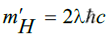 .It is as if this background energy consists of a space field pD(r) consisting of small tiny polarizable dipoles. In that case, the quark's static field can be written as a Poisson equation,
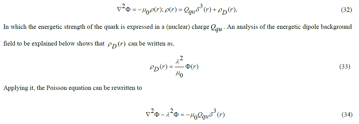
The modification of Poisson’s equation by inclusion of the term λ2Φ is allowed by the relationship between the dipole moment density Pdand the space charge pD(r), [25].
It implies that the dipole moment density is fixed by the parameter λ and the source strength Qu of the quark. Within the range of the source, the dipoles will be polarized, outside the source the dipole direction will no longer be directed, but will be randomly distributed by entropy in all directions. The number of dipoles per unit of volume will remain the same.
Let us proceed by discussing the potential nature of the energetic background field. If an elementary component of the background energy is a Dirac particle of the special type indeed, then it has two real dipole moments. One of the dipole moments μm can be polarized by the quark’s static potential. Its polarizable dipole moment depends on an unknown charge qm and an unknown small mass md . Hence,
As noted above, the decay parameter λ is related to the value of the Higgs boson. This value is derived in the frame of the pion. This frame flies almost at the speed of light. This imposes a relativistic correction λ. To this end, we first write λ as,
If we knew the quark mass, the densityNof energy carriers per unit volume of the background energy could be calculated. On the other hand, if we knewN, we would be able to assess the quark’s “naked” mass.
Now it so happens that vacuum polarization is known in cosmology as well. There is an energetic background field that is responsible for the “dark matter” phenomenon. That dark matter causes objects at the edges of galaxies to orbit their kernels with a significantly faster orbital velocity than calculated by Newton's law of gravitation, even so by including corrections based on Einstein's Field Equation. In 1963, Mordehai Milgrom concluded that this in every known galaxy occurs to the same extent. In the absence of an explanation, he formulated an empirical adaptation to Newton's law of gravitation. This adaptation is characterized by an acceleration constant that is equal for all systems. Its value is 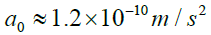 . In 1998, Vera Rubin reported another unexpected cosmological phenomenon. She concluded a more aggressive expansion rate of the universe than the constant rate assumed based on Einstein's Field Equation. Scientists reconciled the latter phenomenon with theory, by assigning a finite value to Einstein’s Lambda (Λ) in the famous Field Equation, which until then had been assumed to have a value of zero. The consequence of this is that the universe must have an energetic background field. Based on cosmological observations of these two phenomena, it has finally been empirically established that the matter in the universe is divided up into three components
 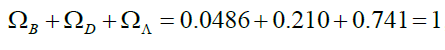 , which are, respectively, the ordinary baryonic matter, the unknown dark matter and the unknown dark energy [26]. It is described how this relationship between these components can be theoretically determined [27].
The key to this is to revise the view that Einstein's Lambda is the cosmological constant as being a constant of nature. In Einstein's 1916 work on General Relativity, this quantity appears only as a footnote with the remark that an integration constant in the derivation is set to zero. See the footnote on p. 804 in [28]. Steven Weinberg in 1972 valued this footnote and promoted this integration constant to the Cosmological Constant [29]. Strictly speaking, though, this quantity is a constant in terms of space-time coordinates. It may depend, in theory at least, on coordinate-independent properties of a cosmological system under consideration (a solar system, a galaxy, the universe) like, for example, its mass. In that case, only at the level of the universe, it is justified to qualify Einstein’s Λ as the Cosmological Constant. In [13] the relationship is derived that,
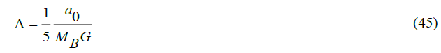
in which Einstein's Λ is found to depend on the gravitational constant G, the baryonic mass MB and Milgrom's acceleration constant a0. Moreover, it turns out that the latter depends on the relative amount of the baryonic mass ΩB in the universe and its Hubble age tH (13.6 Gigayears), such that
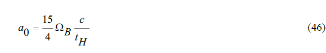
This implies that it is not Einstein's Λ to be regarded as the true Cosmological constant, but that this qualification rather applies to Milgrom's acceleration constant. In this theory, the distribution of the three energy elements of the universe can be traced back to a background energy consisting of elementary components with a “gravitational” dipole moment 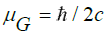 . Within the sphere of influence of the baryonic mass, these are polarized and are by entropy randomly oriented outside it.
Considering that both the nuclear background energy and the cosmological background energy may consist of elementary polarizable components, it would be strange if these components were not the same. The cosmology theory developed in allows to determine the density N of these particles as [13],

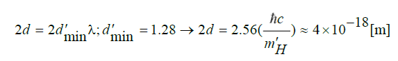
Although at the gravitational level this is an extremely high density, at the nuclear femtometer level (10-15 m) sustaining the hypothesis seems falling short. Nevertheless, if N is used to calculate the bare mass of the quark as deduced above, it turns out that
The dilemma disappears by remembering that volumes should be considered at the wavelength level. Anyhow, that is what Fermi's theory described earlier in this text has taught us. A mass of 1.34 MeV/c2 corresponds to a De Broglie wavelength of 885 fm. That brings us to the picometer level. This is wide enough to consider the background energy effectively uniformly distributed at the quark level. The “naked” mass of the archetype quark as derived in this text depends on six physical quantities. Two of them are generic constants of nature: the vacuum light velocity, and Planck’s constant. Two of them are particle physics related: the mass ratio of the Higgs boson and the weak interaction boson and the rest mass of the pion. Two of them are cosmological: the gravitational constant (a constant of nature) and Milgrom’s acceleration constant (possibly a constant of nature as well).
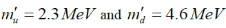
The value thus calculated is of the same order of magnitude as the “naked” mass for the quarks, derived in lattice Quantum Chromodynamics (lattice QCD) from the rest masses of the pion and kaon as m'u=2.3MeV and m'd=4.6MeVcfor, respectively the u quark and the d quark [30]. “Naked” mass has to be distinguished from “constituent” mass, which can be traced back to the distribution of the hadron’s rest mass over the quarks. Because these rest masses are mainly determined by the binding energy between the quarks, the relatively large constituent mass hides the relatively small amount of the true physical “naked” mass that shows up after the removal of the binding energy component. Lattice QCD is based on the Standard Model with (the heuristic) gluons as the carrier of the color force, the (heuristic) Higgs particle as the carrier of the background energy and an interaction model based on Feynman's path-integral methodology. This methodology is based on the premise that in principle all possible interaction paths between the quarks in space-time matter and that the phase difference in transit time of “probability particles” (as a model of quantum mechanical wave functions) over those paths ultimately determines the interaction effect. Such paths can make more or less coherent contributions or completely incoherent contributions. In lattice QCD, the paths are discretized through a grid. This discretization is not by principle, but only intended to limit the computational work that is performed with supercomputers. The strength of this model is its unambiguity because it assumes the application of the principle of least action to a Lagrangian (some authors, therefore, call Lattice QCD a “simple” theory). But it is also the weakness of the model because the (now very complex) Lagrangian is “tuned” to all phenomenological phenomena observed in particle physics and has been given a heuristic mathematical formulation. It is quite conceivable that physical relationships have remained hidden under a mathematical mask. Several examples have been discussed in the two parts of this essay [1].
It might therefore well be that the definition of “naked” mass is model dependent. In the structural model, the pion rest mass is the mass reference. In lattice QCD both the rest mass of the pion and the rest mass of the kaon serve as a reference (in the structural model it is shown that these two rest masses are interrelated). The lattice QCD “naked” mass values are validated from the calculation of the proton mass, but, strictly speaking, this validation only shows the mass relation between the pion and the proton. In [17], it is shown that the structural model is even more accurate in this respect, particularly taking into account its capability for an accurate calculation of the mass difference between a proton and a neutron. It is quite curious that in the PDG listing of quark masses, the formerly used constituent masses of theu,d andsquark are replaced by “naked” masses, while for the other quarks (,cbandt ) the constituent values are maintained. Another curiosity is the mass assignment to the u quark and thed quark in the same ratio as their presumed electric charge. This presupposes that the mass origin is electric. But why should it? And if so, why are these mass values not related by an integer factor with the mass of an electron?
The fact that two different models don’t yield the same value for the indirectly determined unobservable "naked" mass of a quark does not necessarily prove the correctness or incorrectness of one of the two. In neither of the two models, the “naked” mass is used as “the first principle” for mass calculations because the true mass reference is the rest mass of the pion. As long as comparable precisions are obtained, the value of the naked mass is irrelevant in fact. In the end, Occam's knife is decisive in making a choice. Because the “naked” mass value of the quarks as calculated from the dark matter view as developed and summarized in this text rather well corresponds with the mass value of quarks calculated by lattice QCD supports the view that the particle density of the energetic background field constituents is the same for particle physics and cosmology [31]. Denoting these constituents as “darks”, an estimate for their gravitational mass can be derived from the critical mass density of the universe. The critical mass density pc can be expressed in terms of Hubble time tH from the consideration that the universe is a bubble from which light cannot escape: once a black hole, now expanding, where we still live in. Hence it has a (Schwarzschild) radius RS=ctH , such that
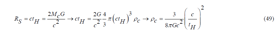
It gives 9.4 10-27 kg/m3. Divided over 1.7 x 1041 particles, it gives a mass of 5.55 10-68 kg per particle, which corresponds to a massive energy of 3 10-32 eV. This makes the darks virtually massless. These particles (“darks”) are polarized (dark matter), randomly oriented (dark energy) or condensed (baryonic mass) [32, 33].
Conclusion
The theory as reviewed in the first part and the second part of this essay gives an unorthodox and anti-dogmatic view of particle physics. It is based on three fundamental issues that have not been recognized and therefore not have been taken into consideration during the development of the Standard Model of particle physics. The first one is the recognition that Dirac’s theory of the electron allows the existence of a particular particle type, which, under a modified set of gamma matrices shows two real dipole moments, instead of a real one and an imaginary one shown by electrons. The second one is the recognition that two of those particles may compose a bond in which their non-baryonic potential energy is converted into a baryonic mass that, under the application of Einstein’s General Relativity Theory, can be conceived as a constituent mass of the two particles.The third one is the awareness of a background field with a uniformly distributed energetic space charge that shields the non-baryonic energy emitted from nuclear wells (quarks). The awareness that the vacuum is not empty has been inherited from a similar awareness in cosmology that since 199 has been invoked to explain the accelerated expansion of the universe under the interpretation of Einstein’s Lambda in his Field Equation. Whereas the Standard Model is essentially descriptive to give an accurate match between experimental evidence and theory, the structural view as described in this essay with its two parts is aimed to show a physical relationship between the many axioms that for mathematical reasons have been introduced in the Standard Model. Among these are concepts such as isospin, the Higgs field, the gluon, SU(2) and SU(3) gauging, etc. In the Standard Model, questions like “Why are there so many elementary particles, why is there such a big mass gap between the (u/d, s, c, b) quarks and the top quark” and why does the lepton stop at the tauon level, have remained unanswered. The usual answer is “It is as it is”.
The reputation of the Standard Model is based upon the claimed accuracy between theory and experiment. That is certainly justified for the QED part. But is it justified for the QCD part as well? Let us take into consideration that “the more axioms, the more accurate a theory is” and that “experimental evidence is usually not hard proof, because many nuclear particles are not observable and can only be detected as “signatures with a theory in mind”.
The structural view exposed in this review allows for the removal of many axioms in the theory by giving it a physical basis, thereby considerably reducing the number of elementary particles.
Even though mass is one of the most relevant attributes of particles, it is probably fair to say that the Standard Model shows a weakness in calculating masses and mass relationships. Particularly here the structural view shows its strength. Furthermore, the structural model allows us to connect particle physics with gravity. In the first part of this essay, it has been shown that the gravitational Constant can be verifiably expressed in quantum mechanical quantities. In this second part, it has been shown how the “dark matter” phenomenon in cosmology is related to the Higgs field phenomenon in particle physics.
Another strength of the structural model, shown in this second part of the essay, is its ability to include neutrinos within its theoretical framework under an explanation of present experimental evidence of their features. How to do so In the Standard Model is an unsolved problem. It is probably fair to say that whereas the Standard Model of particle physics describes the “what”, the structural model describes the “why”.
REFERENCES
- Roza E. From Black-Body Radiation to Gravity: Why Quarks Are Magnetic Electrons and Why Gluons Are Massive Photons. 2023.
- Berryman JM, De Gouvea A, Hernandez D. Solar neutrinos and the decaying neutrino hypothesis. Phys. Rev. D. 2015;92(7):073003.
- Boyarsky A, FrOhlich J, Ruchayskiy O. Self-consistent evolution of magnetic fields and chiral asymmetry in the early Universe. Phys. rev. lett. 2012;108(3):031301.
- Cowan Jr CL, Reines F, Harrison FB, et al. Detection of the free neutrino: a confirmation. Science. 1956;124(3212):103-4.
- Lee TD, Yang CN. Question of parity conservation in weak interactions. Phys. Rev. 1956;104(1):254.
- Wu CS, Ambler E, Hayward RW, et al. Experimental test of parity conservation in beta decay. Phys. Rev. 1957;105(4):1413.
- Bahcall JN, Davis Jr R. Solar neutrinos: a scientific puzzle. Science. 1976;191(4224):264-7.
- Gribov V, Pontecorvo B. Neutrino astronomy and lepton charge. Phys. Lett. B. 1969;28(7):493-6.
- Roza E. On the Flavour States and the Mass States of Neutrinos. 2023.
- Maki Z, Nakagawa M, Sakata S. Remarks on the unified model of elementary particles. Prog. Theor. Phys. 1962;28(5):870-80.
- Roza E. On the second dipole moment of Dirac’s particle. Found. Phys. 2020 ;50(8):828-49.
- Foldy LL. The electromagnetic properties of Dirac particles. Phys. Rev. 1952;87(5):688.
- Comay E. Charges, monopoles and duality relations. Il Nuovo Cimento B (1971-1996). 1995; 110:1347-56.
- Roza E. From Black-Body Radiation to Gravity: Why Neutrinos are Left-Handed and Why the Vacuum is not Empty. 2022.
- Roza E. A hypothetical H-particle. Phys. Essays. 2011;24(1):72-85.
[Google Scholar] [Cross Ref]
- Roza E. The gravitational constant as a quantum mechanical expression. Results phys. 2016; 6:149-55.
- Tanabashi M, Hagiwara K, Hikasa K, et al. Review of Particle Physics: particle data groups. Phys. Rev. D. 2018;98(3):1-898.
- Schafer R, Stöckmann HJ, Gorin T, et al. Experimental verification of fidelity decay: from perturbative to Fermi golden rule regime. Phys. rev. lett. 2005;95(18):184102.
- Griffiths D. Introduction to elementary particles. John Wiley Sons. 2020.
- Christensen CJ, et al., Free-neutron beta-decay half-life. Phys. Rev. D. 1972;5(7):1628.
- "Direct neutrino-mass measurement with sub-electronvolt sensitivity." Nat. Phys.18, no. 2 (2022): 160-166.
- Fukuda S, Fukuda Y, Hayakawa T, et al. The super-kamiokande detector. Nuclear Instruments and Methods in Physics Research Section A: Accelerators, Spectrometers, Detectors and Associated Equipment. 2003;501(2-3):418-62.
- Roza E. On the Mass of the Nucleons from" First Principles".
- Debye P, Huckel E. De la theorie des electrolytes. I. abaissement du point de congelation et phenomenes associes. Physikalische Zeitschrift. 1923;24(9):185-206.
- Gonano CA, Zich RE, Mussetta M. Definition for polarization P and magnetization M fully consistent with Maxwell's equations. Prog. Electromagn. Res. B. 2015; 64:83-101.
- Collaboration P, Ade PA, Aghanim N, et al. AJ. Planck 2013 results. XVI. Cosmological parameters. A&A. 2014;571: A16.
- Roza E. On the vacuum energy of the universe at the galaxy level, the cosmological level and the quantum level.2021.
- Einstein A. Relativity: The Special and General Theory (1916). Estate Albert Einstein. 1961.
- Weinberg S. Gravitation and cosmology . John Wiley Sons Inc. New York. 1972.
- Hashimoto S, Laiho J, Sharpe SR, Particle Data Group. Lattice quantum chromodynamics. Rev. Part. Phys. Ed. by KA Olive et al. (Particle Data Group). 2017; 38:090001.
- Roza E. On the relationship between the cosmological background field and the Higgs field.2020.
- Frieman JA, Turner MS, Huterer D. Dark energy and the accelerating universe. Annu. Rev. Astron. Astrophys. 2008; 46:385-432.
- Peebles PJ, Ratra B. The cosmological constant and dark energy. Rev. mod. phys. 2003;75(2):559.