Research
, Volume: 8( 3) DOI: 10.37532/2320-6756.2020.8(3).198Measuring Planck's Constant Using Light Emitting Diodes
- *Correspondence:
- Mila Bileska
Student, Nova International Schools
Prashka 27 1000 Skopje, North Macedonia
Tel: +38978504141
E-mail: mila.bileska@gmail.com
Received: September 30, 2020; Accepted: October 17, 2020; Published: October 24, 2020
Citation: Bileska M. Measuring Planck‟s Constant Using Light Emitting Diodes. J Phys Astron. 2020;8(3):198.
Abstract
This experiment aims to minimize the margin of error when calculating Planck’s constant (h) using accessible equipment. The study is based on the fact that electromagnetic radiation is quantized and obeys the Planck-Einstein relation. Throughout this experiment, the activation voltage (Vac) and wavelength (λ) of light emitting diodes was measured. To analyze the collected data, two methods were employed. The result from Method 1 was based on analytic calculations, whereas the result from Method 2 was generated through graphical computations. In Method 2, Planck’s constant was represented as a factor of the slope on the λ−1 and Vac linear graph. As hypothesized, Method 2 had a substantially lower margin of uncertainty and yielded a value that had an error of 3.7%. This result is significantly closer to the conventional h when compared to the 5.2% error that was observed in Method 1. However, with respect to the margin of uncertainty, the value of Planck’s constant is within the range of both results. Evidently, the representation of a physical constant as a factor of the slope on a linear graph proved to be a more accurate data analysis method than the analytical averaging of experimental values. This graphical analysis procedure can be employed in various complex physical experiments in order to increase the precision of the final results.
Keywords
Planck-Einstein relation; Planck’s constant; Activation voltage; Margin of uncertainty
Introduction
The significance of Planck’s constant and its measurement
The field of quantum mechanics traces its beginnings to the discovery of the Planck relation. Prior to Planck‟s hypothesis, the Franck-Hertz experiment indicated that light is quantized. By using monoatomic mercury vapor, Hertz monitored the plate current caused by the Hg ions [1]. Accordingly, the first peak in the graphical representation of the results was at 4.9V, which corresponds with mercury‟s spectral line at 253.6 nm [1]. Hereby, although Hertz didn‟t arrive at the conclusion, he demonstrated a fundamental linear relationship between the frequency and energy of light.
After the Franck-Hertz experiment, in an attempt to describe black-body radiation, Planck postulated a theory that radiation energy is transmitted in “quanta” or energy packages. Further, when researching the photoelectric effect, Einstein proposed that light itself is quantized [2]. Hence, the Planck-Einstein relation, or simply the Planck relation, portrays a proportional relationship between the “energy quanta” and frequency (ν) of a photon, through the equation:
Equation 1 calculates the energy (E) of quantized oscillators through multiplying the frequency (ν) with Planck‟s constant (h) of value 6.62607015 × 10⁻³⁴ Js
Planck‟s constant, which applies to quantum oscillators, sets a specific fitting parameter for physical interactions at the quantum scale [3,4] Consequently, it is an integral part of Dirac‟s fundamental quantum condition, qrps − psqr = ihδrs, Heisenberg‟s uncertainty principle, σxσp ≥ h/2 , and the de Broglie relation, λ = h/p [5-7] Most importantly, Planck‟s constant is a parameter determining variable in Schrödinger‟s equation,
in which ψ(x) denotes the wave function, m is the mass, and ℏ represents the reduced Planck constant that has a value of h/2π [8,9]. In essence, Schrödinger‟s equation describes the evolution and present quantum state of a wave function [10]. Consequently, it is used to determine the probabilistic properties of a quantum system, such as the position of subatomic particles [8]. As previously acknowledged, the Schrödinger equation, which is a principle behind all quantum-mechanical phenomena, relies on the Planck constant as a variable that sets the parameter for interactions at the quantum scale.
The CODATA 2017 [11] determined value for Planck‟s constant is 6.62607015 × 10⁻³⁴ Js. Contemporary technology and scientific research have narrowed down the uncertainty regarding this numerical value. Recently, in 2017, D. Haddad et al. published a research article on their experimental results regarding the Planck constant. The experiment detailed one possible procedure for the measurement of h. In summary, the Kibble balance was used to determine the value of hSI/h90, where hSI and h90 are the Planck constant in SI and conventional units, respectively [12]. The value for this relation based on the concluding results is 1.000000236, which implies a high degree of accuracy in the team‟s measurement procedure [12]. For the purpose of quantifying the similarity that the LED experiment has with the conventional value for the Planck constant, the same method of error analysis as in Haddad‟s experiment will be used throughout this paper.
Photodetection noise
Photodetection noise is present when collecting data with a photodiode. It can be observed as small fluctuations in the intensity, value recorded by the light-sensitive detector. Although this occurrence may have many causes, the three major noise sources are categorized as thermal, shot, and dark current noise [13].
Thermal noise, also referred to as the Johnson noise, is generated by the thermal agitation of charge carrying quantum oscillators [14]. As elaborated by Dennis V. Perepelitsa in his theoretical paper, the Nyquist theorem, which was devised in 1928, shows the minimum frequency needed to detect or describe periodic signals and is equal to the sum of energy in the normal modes of electrical oscillation along a shorted transmission line connected to two resistors of resistance R [14]. This noise, which can be calculated through the equation σ2ih = 4kt/RL, (where σ2ih is the thermal noise represented in units of W/Hz, RL denotes the load resistance, T is the absolute temperature, and k represents Boltzmann‟s constant), is faint and detected only through amplification [13]. Consequently, it does not significantly affect the measurements taken with the photodiode in this paper‟s experiment. Shot noise, which is synonymous with quantum noise, is generated by the quantization of the electron‟s charge [14]. In simpler terms, the shot noise is caused by the randomized arrival of photons and therefore, its contribution to the overall measurement, in the case of this experiment, is insignificantly small [15].
Dark current noise is present when no photons interact with the photodiode. Similarly to the previously discussed shot or quantum noise, it can be characterized as white noise [13]. In other words, the dark current noise contains different frequencies with equal intensities.
As examined by Y. Paltiel et al., in their experimental paper "Non-Gaussian dark current noise in p-type quantum-well infrared photodetectors", dark current interference is most commonly a result of the random nature of quantum fluctuations that cause the electrons in the photodiode to get promoted to higher energy levels [16]. Therefore, dark current noise causes the light-sensitive detector to yield an instantaneous positive intensity reading in an otherwise fully dark and isolated environment. Evidently, dark current noise impacts the photodiode reading significantly. Accordingly, as presented in the section “Interpreting the photodiode analog data” below, the dark current interference was monitored and filtered out from the experimental results.
Principle derivations and concepts used in the experiment
Equation 1 demonstrated the Planck-Einstein relation where the term ν refers to the frequency of an electromagnetic wave. Based on the Wavelength frequency relation, ν = c/λ, Planck‟s equation can be modified using the following derivation:
where Vac is the activation voltage of a light emitting diode and qe resembles the elementary charge constant with a value of 1.602176634 ×10⁻¹⁹ C.
All discovered quantum oscillators, including photons and electrons, possess an electric charge equal to the value of the elementary charge constant, qe, or an integer multiple of it [17]. As a result, for the purpose of this experiment, in order to derive voltage from the energy (E), the expression E = Vacqe was used, as shown in Equation 2.
As discussed in section “The significance of Planck‟s constant and its measurement”, electromagnetic radiation is characterized by the wave function, ψ. Consequently, light exhibits wave-like properties. When it passes through a diffraction grating, light separates into its constituent colors. This occurs when the photons pass through the small slits of the diffraction grating. Based on Huygen‟s principle, due to the difference in wavelength of the photons, the constructive and destructive interference of the „newly‟ formed wavelets occurs in different and separate directions [18]. As a result, when visible light passes through the grating, it gets diffracted at a specific angle that can be used to determine the photon‟s wavelength.
Based on the Planck-Einstein relation, the energy required to produce a photon of a specific wavelength is directly proportional to its frequency. Accordingly, in order to calculate Planck‟s constant, the activation voltage of light emitting diodes was measured and converted into units of energy. Equation 1 demonstrates the fact that the energy necessary to produce a photon is an integer multiple of its frequency, where that integer is equal to h. Evidently, by knowing the wavelength (which is equal to c/ν) and activation voltage, Planck‟s constant can be calculated. The purpose of this experimental design is to demonstrate how the margin of uncertainty can be minimized using different data analysis approaches. Although the same numerical points were used, the analytical and graphical calculations yielded varying results. This discrepancy is imperative in experimental research; therefore the experiment was designed to be an accessible demonstration of it.
Experimental Setup
Electronic data collection
For the purpose of this experimental setup, the Arduino Uno electronic board was used. This allowed for a more precise measurement of the output voltage and the intensity reading from the photodiode. The potentiometer, that regulated the voltage throughout the circuit, was connected to the 3.3 V port. As shown in (FIG. 1), it was positioned in a parallel configuration with the light emitting diode; therefore the voltage that passed through the potentiometer directly affected the LED. In this manner the current to the light emitting diode was supplied, regulated, and monitored.

FIG 1: Electronic setup.
Based on the current across the potentiometer, a numerical value was transmitted to the Arduino board, which was automatically translated into a voltage reading. Since the LED and potentiometer were positioned in parallel, the voltage supplied to the light emitting diode corresponded with the measured value from the potentiometer.
The photodiode was independent of the previously discussed circuit. For the purpose of accuracy, the photodiode was positioned 0.5 cm away and facing the LED. The sensor recorded the light intensity that was later graphed, analyzed, and compared with the voltage reading from the potentiometer circuit.
Wavelength measurement setup
The diffraction grating was clamped on a strictly horizontal surface. A directed beam of photons from the light emitting diodes passed through the diffraction grating and was projected on a vertical screen at a specific angle. This screen was equipped with a ruler to measure the distance from the light diffraction projection to the mid-point of the screen (d1). This setup is illustrated in (FIG. 2).

FIG 2: Diffraction grating setup.
Procedure
Usage of the sodium lamp
The sodium vapor lamp is known for emitting photons with a characteristic wavelength of 589.3 nm+0.3 nm [19]. It is classified as a gas discharge lamp [20]. The inner electrical discharge tubes are surrounded mostly by neon and argon gas and traces amount of metallic sodium [21]. The electrical discharge then ionizes the noble gases until the metallic sodium is vaporized from the thermal energy inside the lamp. This process yields monochromatic yellow light with a wavelength of 589 nm+0.6 nm [19]. Accordingly, throughout this experiment, the sodium vapor lamp was used to calibrate the wavelengths.
Wavelength measurement procedure
The wavelength measurement procedure was repeated multiple times in order to maximize the accuracy of the results. As shown in (FIG. 2), the beam of light from the LED passed through the linear diffraction grating and got projected on the screen at a specific angle, θ.
To measure θ, the inverse tangent function was taken from the ratio d1/d2, where d1 is the distance from the midpoint of the screen to the diffracted light intersection point (represented by the horizontal dashed line on FIG. 2), and d2 is the distance from the screen to the diffraction grating (represented by the vertical dashed line on FIG. 2) in meters. This calculation generated the diffraction angle; θ. Throughout this process, the used length measuring device was known to have a margin of error of 0.05 cm. This value was used in the error analysis alongside data that was collected through multiple trials.
Further, to finalize the computation of the photon‟s wavelength, the ratio of ddg/sinθ was calculated, where ddg is the distance between individual lines in the diffraction grating. This ratio yielded a numerical value for the wavelength in meters. Multiple trials were conducted and an average value of the wavelength for each light emitting diode was found.
Voltage measurement procedure
The activation voltage was measured in a fully dark environment. The same setting was used for each LED. The elimination of external light sources caused the photodiode to detect the first photon(s) with a higher degree of accuracy. Moreover, this ensured that the light-intensity reading will not display unaccounted photo detection noise. As noted in section “Electronic data collection”, the photodiode was positioned in close proximity to the LED to maximize the calibration and accuracy of the results.
The voltage supplied to the light emitting diodes was manually increased by the potentiometer. Initially, the voltage was 0.00 V and was gradually amplified to a value of 3.3 V. Multiple trials were conducted to ensure the accuracy of the findings.
The value for the voltage was recorded on a time interval of 100 milliseconds which translated to an increase of 0.05 V between measurements. In parallel, the intensity data from the photodiode was paired up with the corresponding voltage value. As discussed in section “Activation voltage results”, to analyze the findings, a graphical representation of the data was created, with the voltage as a control variable. The graph in (FIG. 3), depicts the photodiode intensity reading as a function of the voltage.

FIG 3: Activation voltage comparisons.
Interpreting the photodiode analog data
As discussed in section “Photodetection noise”, the dark current of the photodiode adds noise to the intensity. Accordingly, prior to the voltage measurement, the photodiode was set to collect data in an unlit environment. This yielded a graphical representation of the photodetection (or dark current) noise as shown in (FIG. 4). This was later taken into account when the photodiode data was being analyzed.

FIG 4: Dark current noise graph.
The data presented in (FIG. 4) was normalized for the purpose of this experiment. Moreover, each data-point was taken on a time interval of 100 milliseconds. As seen above, the amplitude of the photodetection noise did not exceed 2 units in either direction. These findings were taken into consideration when calculating the margin of error of the voltage measurements, as well as the final results.
Tabular and Graphical Data with an Analysis of Uncertainty
Wavelength results
TABLE 1 shows the calculated results for the wavelength of each light emitting diode. The margin of error was determined experimentally by conducting and averaging the results from 10 trials for each LED, as well as through calculus-based computations with the known uncertainty values of the measuring devices.
TABLE 1. Wavelength of LEDs.
| Color of LED | Wavelength (nm) |
| Red | 627 ± 30 |
| Yellow | 576 ± 50 |
| Green | 534 ± 25 |
| Blue | 490 ± 20 |
Activation voltage results
FIG. 3 is a graphical representation of the collected data with the photodiode and Arduino setup. As shown in FIG. 3, the photodiode reading was graphed as a function of voltage, which were the independent and controlled variables in the experiment. Notably, the photodiode intensity had no specific units and were normalized for the purpose of comparison. Hence, the lowest recorded intensity value was substituted with the integer "1" and further readings were adjusted accordingly.
The relative concave-down curves of the graph are the result of the photodiode‟s spectral response. Terubumi Saito in his experimental work, "Spectral Properties of Semiconductor Photodiodes", outlines the reactivity curves of different light sensitive detectors [22]. The graphical representation of the sensitivity data from Si Photodiode (B), which Saito depicts in his paper, is in correspondence with the observed spectral response of the photodiode used for generating the data from FIG. 3 [23]. Hereby, the relative distance between the curves in FIG. 3 is due to the photodiode‟s greater sensitivity at longer wavelengths (600 nm to 700 nm). As a result, photons of longer wavelengths, that produce red light, were detected with a greater intensity than the blue or green LED.
Based on the results generated by multiple trials, the margin of error was determined to be ± 0.1 V. The following TABLE 2 shows the activation voltage Vac for the light emitting diodes.
TABLE 2. Activation voltage for LEDs.
| Color of LED | Activation voltage (V) |
| Red | 1.83 ± 0.10 |
| Yellow | 1.98 ± 0.10 |
| Green | 2.25 ± 0.10 |
| Blue | 2.47 ± 0.10 |
Calculations for the Planck constant (Method 1)
As demonstrated in section “Principle derivations and concepts used in the experiment” through Equation 2, the Planck‟s constant, h, can be calculated by determining the activation voltage, Vac, and wavelength of the photons produced by the light emitting diodes. This calculation, however, includes an assumption that the experiment is carried out in a vacuum. Accordingly, the calculations used qe, or the elementary charge constant, and c, or the speed of light, that have the values of 1.602176634 × 10⁻¹⁹ C and 299792458 m/s, respectively [11]. The following TABLE 3 portrays the manually calculated results for the Planck constant. This calculation relies on Equation 2 and the results from sections “Wavelength results” and “Activation voltage results”. For the purpose of clarity, these results will be referred to as Method 1.
Referring back to section “The significance of Planck‟s constant and its measurement”, it was elaborated that the value of hSI/h90, where hSI and h90 are the Planck constant in SI and conventional units, respectively, was used as a method of determining the result‟s numerical accuracy. Based on TABLE 3, the value of hSI/h90 for this experiment was calculated as 1.055254. This implies that the final results have a high degree of correspondence with the predetermined value of Planck‟s constant. In addition, the percentage of error was calculated to be ≈ 5.236%. The greatest deviation from the value for the Planck constant was observed with the yellow LED, with a percentage error of ≈ 8.014%. However, the measurements with the blue light emitting diode had an accuracy of ≈ 97.62%. This is the due to the faintness of the yellow LED‟s light when compared to the blue, which made the wavelength measurements less accurate, as reflected by the error analysis in TABLE 1.
Establishing a graphical relationship (Method 2)
In this section, the fundamental inversely-proportional relationship between the wavelength and activation voltage of light emitting diodes is further demonstrated through the following graph. For the purpose of clarity, this procedure will be referred to as Method 2.
FIG. 5 is a representation of the data collected throughout this experiment. The chosen values on the axis are the result of Equation 2. In particular, Equation 2 was modified to resemble the formula of a linear function, y=mx+b, where m is the slope and b is the intercept. To enhance the accuracy of the best-fit line, based on convention, the values (0,0) were added. Throughout this process, the following derivation was used:
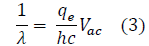

FIG 5: Best-fit line of the linear relationship between 1/λ and V.
Further, based on the linear formula, it is evident that the slope, or "m", is equal to qe=hc.
In FIG. 5, the best-fit line has the formula of: y = 837870.1449315293 × -19490.121828835643. By knowing the mean slope (m), Planck‟s constant can be calculated through the following equation:
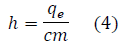
where m ≈ 837870.1449.
As hypothesized, the value for the Planck constant calculated in this manner was 6.378 ×10⁻³⁴ Js, which is highly similar to the results generated through Method 1, presented in TABLE 3. To demonstrate exactly, the similarity between the results is 98.45%. As discussed through section “Final Results”, this discrepancy is caused by the numerical estimation that took place in Method 1. As a result, the least square fit slope calculation yielded a more precise value for h.
TABLE 3. Manual calculations for h (Method 1).
| Color of LED | Result for h (Js) |
| Red | 6.132 × 10⁻³⁴ ± 0.628 × 10⁻³⁴ |
| Yellow | 6.095 × 10⁻³⁴ ± 0.837 × 10⁻³⁴ |
| Green | 6.421 × 10⁻³⁴ ± 0.586 × 10⁻³⁴ |
| Blue | 6.484 × 10⁻³⁴ ± 0.526 × 10⁻³⁴ |
| Average | 6.279 × 10⁻³⁴ ± 0.644 × 10⁻³⁴ |
| Percentage error | 5.24% |
Final Results
Tabular display and comparison
Based on what was presented in section “Tabular and graphical data with an analysis of uncertainty”, the graphical method of determining Planck‟s constant has yielded a more accurate result. This is due to the fact that the process of analytical calculation includes estimation and decimal rounding, whereas FIG. 5 was generated through advanced Python computational software. The following TABLES 4 and 5 displays the findings alongside the percentage of error and margin of uncertainty.
TABLE 4. Results: Planck’s constant.
| Manual computation value (Method 1) | Graphical value (Method 2) |
| 6.279 × 10⁻³⁴ | 6.378 × 10⁻³⁴ |
| ± 0.644 × 10⁻³⁴ Js | ± 0.312 × 10⁻³⁴ Js |
TABLE 5. Results: Comparison.
| Method | Percentage error (%) | hSI/h90 Value |
| Method 1 | 5.237 | 1.0552 |
| Method 2 | 3.742 | 1.0389 |
Notably, with respect to the margin of uncertainty, the calculation from Method 1 can be anywhere from ≈ 5.635 × 10⁻³⁴ Js to ≈ 6.923 × 10⁻³⁴ Js, whereas the result of Method 2 can range from ≈ 6.066 × 10⁻³⁴ Js to ≈ 6.69 × 10⁻³⁴ Js. Significantly, the conventional value of Planck‟s constant, 6.62607015 × 10⁻³⁴ Js, is within the range of both results, with Method 2 providing a more precise value.
Discussion
Planck‟s constant is fundamental to the understanding of quantum physics since it is closely related to the properties of the vacuum. Moreover, it outlines the principles behind the quantization of light and energy by implying that the elementary wave packet has a critical size and gets transmitted through the allornone principle [4]. Consequently, this gives the known Planck-Einstein relation its linear properties, since energy is equal to an integer multiple of the base frequency.
The main purpose of this experiment was to demonstrate accessible, yet accurate procedures for measuring the fundamental Planck constant. Although this experimental setup yields a percentage error of 3.742% (or 5.237% for the manual calculation), it is an efficient method of determining the value of Planck‟s constant and verifying the fundamental Planck-Einstein relation represented through Equation 1. As a result, this procedure can be replicated in almost any lab setting with minimal equipment. Most importantly, this experiment provides a thorough comprehension of the fundamental quantum behaviour of the photon.
An important aspect of this experiment is the margin of uncertainty that is higher for Method 1. Although the same data points for the activation voltage and wavelength were used, the graphical calculation had a lower uncertainty value. For Method 1, the uncertainty was calculated manually for each LED through the differential equation  This was then averaged to a value of ± 0.644 × 10⁻³⁴ Js as shown in TABLE 4.
On the other hand, Method 2 does not treat each data point separately, but rather automatically minimizes the standard deviation which is depicted by the best-fit line in FIG. 5. Due to the relation between the slope, m, and Planck‟s constant, the margin of uncertainty can be represented by 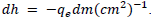 Hereby, this equates to ± 0.312 × 10⁻³⁴ Js. Evidently, this method reflects only the collective uncertainty of the data points.
As expected, due to the higher precision rate observed for Method 2, the final result was more accurate than the one produced through manual calculation.
To further reduce the margin of uncertainty, the electronic Arduino Uno board can be programmed to automatically increase the voltage, using smaller intervals between sensor measurements. This will significantly reduce the margin of uncertainty in the activation voltage measurements. Moreover, the accuracy of the results will be increased if a photodiode with a wider and more evenly distributed spectral response is used alongside LEDs with an amplified photon beam. However, these additions will increase the equipment cost for the experiment.
The comparison of both methods demonstrates how different data analysis approaches can yield more (or less) accurate results. When measuring physical constants that are related through complex equations to the controlled variables of the experiment, a graphical representation allows for more precise calculations. Evidently, the representation of a constant as a factor of the slope on a linear graph that passes through the origin would prove more accurate than analytically averaging the experimental values. This graphical analysis method can be employed in simple experiments, such as calculating g, as well as more complex, such as the determination of qe, in order to increase the precision of the final results.
The results conclusively demonstrate that there is an underlying fundamental linear relationship between the energy required to produce a photon and its frequency (which can be represented through the derivation c/λ). Although this has been verified through numerous experiments that utilize advanced technological equipment, the method outlined throughout this study is considerably more accessible and with a low percentage of error. Importantly, as previously acknowledged, this procedure can be replicated in any laboratory setting with minimal equipment.
Conclusion
The data presented in section 5 indicates that there exists a linear correlation between the wavelength and activation voltage of light emitting diodes. Therefore, Planck‟s constant can be calculated both graphically and through analytical computations as shown in section “Tabular and graphical data with an analysis of uncertainty”. The analysis of this data confirms the Planck-Einstein relation which implies that light is quantized and travels in energy packages, or quanta.
Based on the data from section “Final results”, it is evident that Method 2, or the computer-generated best-fit line, is more accurate in calculating the Planck constant. Although the same data points were used throughout both procedures, the final calculations differ due to the estimation and lower precision rate observed in Method 1.
Overall, however, both analysis methods proved effective in determining Planck‟s constant. The similarity between the results was calculated to be 98.45%. Method 2 yielded a substantially similar value to the conventional h with a percentage error of 3.742%. With respect to the margin of uncertainty, the conventional value for Planck‟s constant, 6.62607015 × 10⁻³⁴ Js, is within the upper range of both results.
Acknowledgements
I want to express gratitude to my mentor Prof. Jenny Magnes.
References
- https://www.researchgate.net/publication/312042429_Franck_-_Hertz_Experiment.
- Planck M. On the theory of the energy distribution law of the normal spectrum. Dtsch Phys Ges. 1900;2:1-8.
- Boyer TH. The contrasting roles of Planck's constant in classical and quantum theories. Am J Phys. 2018;86:280-3.
- Chang DC. Physical interpretation of Planck's constant based on the Maxwell theory. Chinese Phys. 2017;26:040301.
- Broglie L. Recherches sur la theorie des quanta. 1924
- http://digbib.ubka.uni-karlsruhe.de/volltexte/wasbleibt/57355817/57355817.pdf.
- https://en.wikipedia.org/wiki/Interferometry.
- https://www.ligo.caltech.edu/video/ligo20160211v2.
- Gurzadyan VG, Ozernoy LM. Accretion on massive black holes in galactic nuclei. Nature. 1979;280:214-5.
- https://en.wikipedia.org/wiki/Accretion_disk.
- https://codata.org/initiatives/strategic-programme/fundamental-physical-constants/.
- Haddad D, Seifert F, Chao LS, et al. Measurement of the Planck constant at the National Institute of Standards and Technology from 2015 to 2017. Metrologia. 2017;54:633.
- Hui R. Introduction to fiber-optic communications. Elsevier/Academic Press, 2020.
- https://web.mit.edu/dvp/Public/noise-paper.pdf.
- https://web.ece.ucsb.edu/Faculty/rodwell/Classes/graduate_noise_class/noise_notes_set7_new.pdf.
- Paltiel Y, Snapi N, Zussman A. Non-Gaussian dark current noise in p-type quantum-well infrared photodetectors. Appl Phys Lett. 2005;87:231103.
- Millikan RA. On the elementary electrical charge and the Avogadro constant. Phys Rev. 1911;32:349-97.
- Wu XY, Zhang BJ, Yang JH, et al. Quantum theory of light diffraction. J Mod Opt. 2010;57:2082-91.
- Hossain MM, Pant T, Vineeth C, et al. Daytime sodium airglow emission measurements over trivandrum using a scanning monochromator: First results. Annales Geophysicae. 2010;28:2071-7.
- http://lampes-et-tubes.info/doc/Electric_Discharge_Lamps.pdf.
- Rennie R, Law J. Sodium-vapour lamp. A dictionary of physics. Oxford University Press, 2019.
- Saito T. Spectral properties of semiconductor photodiodes. Advances in Photodiodes. 2011;1:3-24.
- Nyquist H. Thermal agitation of electric charge in conductors. Phys Rev. 1928;32:110.