Original Article

, Volume: 11( 4) DOI: 10.37532/2320-6756.2023.11(4).335

• View PDF
• Download PDF

Flyby Radio Doppler and Ranging Data Anomalies are due to different inbound and outbound velocities in the CMB rest frame

*Correspondence:

Roland Pabisch
Independent Researcher, Austria,
E-mail: roland.pabisch@liwest.at

Abstract

The COBE, WMAP, and Planck data analyses exhibit that the CMB rest frame can be seen as a fundamental, absolute space, the CMBspace. All Earth flyby radio Doppler data anomalies can be resolved by applying the general, classical Doppler formula (CMB-Doppler formula) of first order for two-way signals between earthbound Deep Space Network stations and a spacecraft during an Earth flyby. For that purpose, the annually varying absolute velocity vector ue of Earth is used, derived from the absolute velocity vector of the solar system barycenter, usun magnitude 1 369.82 0.11 sun u kms  , in direction of constellation Crater, near Leo. Together with the relative,asymptotic inbound and outbound velocity vectors inv and outv in the equatorial frame, we obtain the absolute inbound and outbound velocity vectors uin and uout in the equatorial frame. The relative, asymptotic inbound and outbound velocities are actually equal in magnitude( ) in out v  v , while the magnitudes of the absolute inbound and outbound velocities of a spacecraft are in general different ( ) in out u  u , leading to the apparent anomaly. Thus the use of the CMB-Doppler formula explains the so far as residual considered positive or negative differences in energy. The measured, different absolute velocities in the CMB rest frame explain the supposed radar ranging data residuals as well.

Keywords

Earth flyby anomalies; Absolute velocities in the CMB rest frame; General classical Doppler formula of first and second order in the CMB rest frame

Theoretically Derived Formula is Reproducing the Empirically Devised Prediction Formula

The flyby anomalies, which in most cases show an apparent acceleration, some null results and one significant deceleration between the inbound and outbound flights, are still unexplained [1, 2]. The total geocentric orbital energy per unit mass should be the same before and after the flyby at infinity. The data indicate this is not always true.

To predict further flyby anomalies, 15 years ago (Anderson & Campell & Ekelund, 2008) published an empirically devised formula from previous flyby anomaly data, which involves the incoming and outgoing geocentric latitudes of the relative, asymptotic velocity vectors [1],

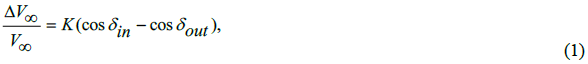
where ΔV_∞ is the apparent anomalous difference in velocity, V_∞ is the asymptotic relative velocity, δ_in is the asymptotic, geocentric latitude of the inward flight trajectory, δ_out is the asymptotic, geocentric latitude of the outward flight trajectory, and K has the constant value 3.099×10^-6 . Using the CMB-Doppler formula approach for two-way tracking signals (see formulas (2) and (3)), we obtain K_CMB = 3.059 [3]. Obviously, the ranging data anomaly is also caused by the different absolute velocities of the inbound and outbound flights, see FIG. 1, and again the CMB-approach will explain accelerations, decelerations and null results as well.

The latest Planck dipole data analyses Planck Collaboration I indicate a peculiar velocity of the solar system of 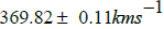in direction of constellation Crater near Leo, at 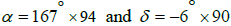. The absolute velocity of Earth in the CMB rest frame varies between u_e = 340kms^-1 around mid-June and u_e = 400kms^-1 around mid-December during the yearly revolution, while the velocity at mid-March or mid-September is u_e = 371kms^-1 . From that velocity the value K_CMB = 3.059 10^-6 follows, if the CMB-space approach is applied, see formula (9).

We now assert, that calculating the frequencies of two way signals between any two moving bodies in the universe, especially in the solar system, the CMB-Doppler formula of first order in the absolute space of the CMB rest frame has to be applied, instead of the relativistic Doppler formula of first order. The absolute velocity of a Spacecraft (SC) is derived by addition of its relative velocity in the geocentric frame together with the absolute velocity of Earth, see FIG. 1. The absolute velocity of the Deep Space Network stations (DSN) is calculated by adding its rotational velocity in the geocentric frame and the absolute velocity of Earth. We neglect the rotational velocity in our formula for simplicity because of the minimal effect, hence . The time dilatation effect as a function of absolute velocities in the CMB rest frame is neglected too, for reasons we discussed in Pabisch & Kern, and in a more recent paper [4, 5, 6]. All vectors are defined in the equatorial frame of Earth.

The CMB-Doppler formula of first order for an uplink signal reads,

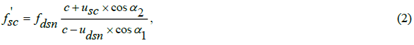
where f_dsn denotes the frequency of the uplink signal emitted by a DSN station, f^'sc the frequency of the uplink signal received and measured by a spacecraft SC, c the constant velocity of light in the CMB rest frame, α₁ the angle between the vector and the vector of the uplink signal, α₂ the angle between the vector and the vector of the downlink signal.

The CMB-Doppler formula of first order for a downlink signal reads,

where denotes the frequency of the downlink signal, as received and measured by a DSN station.

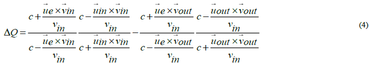
We assume that in the geocentric frame the condition v_in = v_out at infinity is valid, despite the apparent flyby anomaly, and the relative and absolute velocity vectors of formula (4) are defined as,

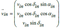
is the relative, asymptotic velocity vector of the incoming spacecraft, as calculated in the equatorial frame,

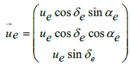
is the absolute velocity vector of Earth in the equatorial frame,

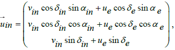
where 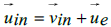is the absolute, asymptotic velocity vector of the incoming spacecraft in the equatorial frame,

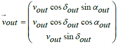
is the relative, asymptotic velocity vector of the outgoing spacecraft, as calculated in the equatorial frame, and

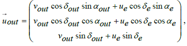
where 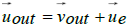is the absolute, asymptotic velocity vector of the outgoing spacecraft in the equatorial frame.

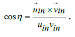
Each of these vectors is defined in the equatorial frame of Earth by means of its declination δ and right ascension α and its magnitude relative to the center of Earth. Furthermore ϑ is the angle between the absolute velocity vector of the geocentric, and the relative, asymptotic velocity vector of the incoming spacecraft, as calculated in the equatorial frame,

where

γ denotes the angle between the absolute velocity vector , and the relative, asymptotic velocity vector of the outgoing spacecraft in the equatorial frame,

where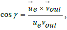

ε denotes the angle between the absolute, asymptotic velocity vector of the outgoing spacecraft, and the relative, asymptotic velocity vector of the outgoing spacecraft in the equatorial frame,

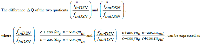
From formula (4) we now obtain formula (5),

where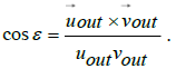

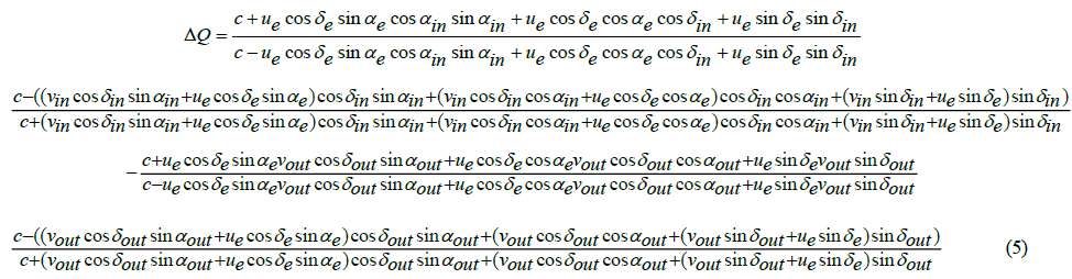
Since the asymptotic inward flight right ascension angle α_in, and the asymptotic outward flight right ascension angle α_out do have a negligible effect on the quotient ΔQ of α_in formula (5), we approximate further, and by equating α_in = α_out=α_e =δ_e we obtain with

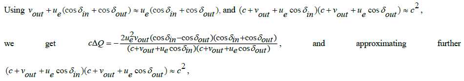
we obtain,

If we consider as difference in velocity, we get,

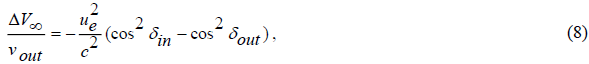
and finally,

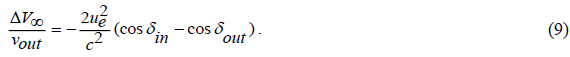
The term yields 3.059×10^-6 for the factor K_CMB , if the velocity of Earth u_e = u_dsn = 371kms^-1 around mid-March is inserted. Due to the CMB-approach, the value of 3.059×10^-6 is not constant, but varies as a consequence of the annual variation of the absolute velocity of Earth between u_e = 340kms^-1 and u_e = 400kms^-1 . Around mid-June K_CMB = 2.57× 10^-6 results, and around mid- December K_CMB = 3.55 × 10^-6 . The negative sign of our factor KCMB stems from the difference of the absolute inbound velocity minus absolute outbound velocity as can be seen in formula (4). The other way around a positive value results.

Cahill derived a formula on equivalent theoretical reasoning. He asserted, that the speed of light is not invariant, and is isotropic only with respect to the CMB rest frame [7]. For some reason he then applies a shibboleth absolute velocity of the solar system to calculate the flyby effects, which deviates significantly in direction and magnitude from the latest Planck values.

Note that the formula by Anderson et al., and hence our theoretically derived formula as well, gives wrong, not null anomaly predictions for the second and third Rosetta flybys, and for the Juno flyby of October 2013, [1, 2]. A deviation sometimes arises when the inbound frequency, in fact due to the absolute inbound velocity u_in , leads to a misleading value of the relative inbound velocity v_in , which results from the standard Doppler formula of first order and the varying factor K_CMB may be a reason, too. The difference between the inbound angles of the relativistic Doppler formula and the CMB-Doppler formula should not be overlooked also, see FIG. 1.

Predictions

The dipole Doppler term of 1st order is the result of the motion of our solar system through space. It is a frame dependent quantity, and we can determine the absolute rest frame as that in which the dipole would be zero. We conclude from formula (9), and the resulting factor K_CMB , that the use of the CMB-Doppler formulas does yield frequencies which will match all measured positive or negative deviations during Earth flyby maneuvers, despite v_in = v_out is valid in the geocentric frame. A renewed evaluation of the correspondently observed ranging data, using the magnitudes of the absolute, asymptotic inbound and outbound velocity vectors, and of the absolute velocity vector of Earth will exhibit velocity differences which explain the seemingly anomalies, measured during some flyby man oeuvres. Several other successful applications of the CMB approach make a random match of formula (9) with the empirically found formula (1) vastly improbable.

The motion of an observer with velocity v relative to the isotropic Planckian radiation field produces a temperature pattern of [10, 11],

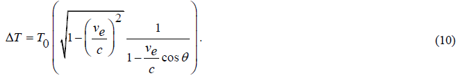
Formula (10) is written in most publications,

Thus hiding the effect of time dilatation in CMB-space, often described as Doppler Effect of 2^nd order which is a function of velocity too, but a quite different physical effect compared to the 1^st order effect. The value of the quadratic term of the CMB dipole formula (10), the inverse γ-Factor, precisely confirms the purely kinematic origin of the first order effect. That concordance indicates we have to interpret the time dilatation effect as an asymmetric function of absolute velocities u in the CMB rest frame [5]. Due to v_e = v_u in formula (10) and (11), Earth Eigen time is obviously not invariant since it varies annually around a time dilatation value of 765nss^-1 at mid-March or mid-September. Clocks at Earth are delayed less than one microsecond per second versus a clock at rest in the CMB-rest frame, the SI-second is not invariant. Only against the absolute temperature variations, due to the absolute motion of Earth that asymmetric effect can be measured, not within any laboratory on Earth, at least until now [12].

The CMB Doppler formulas of 1^st order not only allow to calculate the, in general slightly different, absolute inbound and outbound velocities of flyby man oeuvres, thus resolving the flyby anomalies. The quite different phenomenon of the annual and diurnal signal residuals on top of the resolved Pioneer 10 acceleration term is as well resolved by applying the CMB Doppler formula of 1^st order [6,8, 9].

The CMB multipole anomaly is resolved in CMB-space as well. The observed alignment of the low multipoles (quadrupole and octopole) with one another and their perpendicular orientation to the Ecliptic is not a mysterious property of the presumptive background radiation [13-15]. That in standard physics unexplained phenomenon is caused by the annual motion of Earth, and the fortunate random fact, that the absolute vector of the solar systems velocity runs nearly parallel to the ecliptic, near to the equinoxes. Summarizing, we have several independent indications that the CMB-space approach is new physics:

• We can measure absolute velocities and absolute directions of bodies, stars and galaxies, at least in our cosmic neighborhood.

• The application of the classical Doppler formula of 1st order in the CMB-space (CMB Doppler formula) resolves several different, so far unexplained deviations from the standard Doppler formula of 1^st order.

• Absolute velocities of bodies cause physical effects like time dilatation. That supports the assumption of an inertial mass of photons [5], [6].

• The solar system is not cosmically aligned, as argued in [13-15], and the CMB anomaly of the north-south hemispheric asymmetry, the preference of odd parity, and the cold spot are all resolved in an anisotropic and inhomogeneous cosmos.

Conclusion

We predict, the forthcoming data and images from the James Webb Space Telescope (JWST) will show that the expected structures and traces of an infant universe, according to the ΛCDM model are not to find in the outermost regions. Instead, at least some massive galaxies and quasars will show up in the data. Possibly the region beyond a distance of 13.7 billion years is not the assumed edge of our Universe. The presumptive age of our cosmos of 13.8 billion years is challenged, just a several other components of the ΛCDM model. The particular reasons, supporting those predictions, will follow in another publication.

References

1. Anderson JD, Campbell JK, Ekelund JE, et al. Anomalous orbital-energy changes observed during spacecraft flybys of Earth. Phys. Rev. Lett. 2008;100(9):091102.

   [Google Scholar] [Crossref]

2. Acedo L. The flyby anomaly: a multivariate analysis approach. Astrophys. Space Sci. 2017;362(2):42.

   [Google Scholar] [Crossref]

3. Pabisch R., Kern Ch. Verfahren zur Verbesserung der Steuerungsgenauigkeit einer Raumsonde im Sonnensystem. Deutsches Patent- und Markenamt, DE 10 2010 054741 A1; 2010 [Google Scholar] [Crossref]
4. Aghanim N, Akrami Y, Arroja F, et al. Planck 2018 results-I. Overview and the cosmological legacy of Planck. Astron. Astrophys. 2020;641:A1.

   [Google Scholar] [Crossref]

5. Pabisch R. Derivation of the time dilatation effect from fundamental properties of photons. Springer-Verlag Wien New York, Linzer Universit¨atsschriften. 1999;ISBN 3-211-83153-3 [Google Scholar] [Crossref]
6. Pabisch R.,Residual annual and diurnal periodicities of the Pioneer 10 acceleration term resolved in absolute CMB rest frame. viXra:1806.0389v1. Astrophysics, 2018 [Google Scholar] [Crossref]
7. Cahill RT. Resolving spacecraft Earth-flyby anomalies with measured light speed anisotropy. Prog. Phys. 2008;3(6):9-15.

   [Google Scholar] [Crossref]

8. Anderson JD, Laing PA, Lau EL, et al. Study of the anomalous acceleration of Pioneer 10 and 11. Phys. Rev. D. 2002;65(8):082004.

   [Google Scholar] [Crossref]

9. Rievers B, Lämmerzahl C. High precision thermal modeling of complex systems with application to the flyby and Pioneer anomaly. Annalen der Physik. 2011;523(6):439-49.

   [Google Scholar] [Crossref]

10. Adam R, Ade PA, Aghanim N, et al. Planck 2015 results-VIII. High Frequency Instrument data processing: Calibration and maps. Astron. Astrophys. 2016;594:A8.

    [Google Scholar] [Crossref]

11. D. Scott, G.F. Smoot 29. Cosmic Microwave Background, 2019. [Google Scholar] [Crossref]
12. Sanner C, Huntemann N, Lange R, et al. Optical clock comparison for Lorentz symmetry testing. Nature. 2019;567(7747):204-8.

    [Google Scholar] [Crossref]

13. Schwarz DJ, Copi CJ, Huterer D, et al. CMB anomalies after Planck. Class. Quantum Gravity. 2016;33(18):184001.

    [Google Scholar] [Crossref]

14. Schwarz D.J, Starkman G.D, Huterer D, et al. Is the low-l Microwave Background Cosmic? Phys. Rev. Lett. 2004.[Google Scholar]

    [Crossref]

15. Huterer D. Why is the solar system cosmically aligned?.2007 [Google Scholar] [Crossref]