Mini Review
, Volume: 11( 9) DOI: 10.37532/2320-6756.2023.11(9).377Estimation of Derivatives by the Method of Differenceless Derivatives
- *Correspondence:
- Y Mahotin
Department of Astronomy,
Stanford University,
Stanford,
California,
United States,
Tel: 14084200962;
E-mail: yuri.mahotin@yahoo.com
Received: April 14, 2023, Manuscript No. TSPA-23-95768; Editor assigned: April 17, 2023, PreQC No. TSPA-23-95768 (PQ); Reviewed: May 02, 2023, QC No. TSPA-23-95768; Revised: June 14, 2023, Manuscript No. TSPA-23-95768 (R); Published: June 21, 2023, DOI: 10.37532/2320-6756.2023.11(9).377
Citation: Mahotin Y. Estimation of Derivatives by the Method of Differenceless Derivatives. J Phys Astron. 2023;11(9):377
Keywords
Derivative; Numerical algorithm; Technology; Extrapolation; Prediction
Introduction
Derivatives and especially numerical derivatives are widely used in mathematics, physics, applied sciences and almost everywhere where there is a need for this. The first and second derivatives, known as speed and acceleration are used almost everywhere, while the third, fourth, fifth and sixth derivatives are used very rarely in special applications, higher order derivatives are never used anywhere [1-3]. And there are several reasons for this; in the future we will consider only numerical derivatives. Firstly, everything rests on the fact that it is very difficult to calculate derivatives of a higher order. Secondly, there is no theory and applications that use higher order derivatives, which follows from the first reason. Forward, backward and central differences are commonly used to calculate derivatives and require the function f (x) to be evaluated with an equidistant step h, f (x+h), which may not be possible if the data comes from a measurement [4,5]. In addition, the step size must be very small, which again may not always be feasible. To solve the above problems, we have developed a new algorithm called differenceless derivatives to calculate derivatives from the first to the n-th, where n can be very large 10, 100 and even 100000 and there is no need to have a small step h, the step h can be big and non-equidistant [6].
Literature Review
The method of differenceless derivatives: Consider smooth n times differentiable function f (x) then the function f (x) at point (x+h) can be approximated by Taylor series:
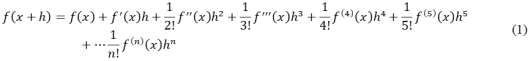
If at the point x all derivatives from the first to the nth are known, it is easy to calculate the value of the function at any point x+h, such a problem is called the direct problem. However, we will be interested in the inverse problem: on the set of points x+hi, (1<i<m) the values of the function f (x+hi) are given to find the values of the derivatives f(x) at point x. For the sake of convenience, we introduce the following notation: Δf(h)= f (x+h)-f (x),Y͞T= (y1, y2.....yn)T= (f '(x), f '' (x).....f(n) (x))T, then equation
(1) can be written in the following form:

This linear equation with respect to the unknown vector y must hold for any values of h, such a requirement for this equation leads us to a system of linear equations written in matrix form as:

Where the quadratic matrix (n × n) A is a function of hi, i.e. A(hi) and the vector b is a function of ΔA(hi) and hi, i.e. b=b(Δf(hi), (hi). The solution of the equation (3) is: y =A-1b, which represents the values of the derivatives from the first to the nth, for that reason the algorithm is called differenceless derivatives. A distinctive feature of this algorithm is that it is impossible to calculate; for example, only the first derivative, all derivatives will be calculated and as a consequence of this, since all components of equation (2) are included in the calculations, the accuracy of calculating the derivatives is much higher than in calculations using, for example, central differences. Another advantage of the differenceless derivatives algorithm is that the requirements for the step size h are reduced, so if the optimal step size h for the forward differences is about 1e-7, then the differenceless derivatives algorithm can use a value of 0.1 and even more, which is very necessary if the data comes from measurements. In what follows, we will refer to all data used as measured data.
To test the new differenceless derivatives algorithm, we developed a Linux program written in C called dld (differenceless derivatives). Matrix A is a dense matrix, so we chose the Gauss-Jordan elimination algorithm as a linear solver. The input parameters of the program are the values of the function at the point x, at which the derivatives will be calculated and at all points x+hi, (1<i<m) presented in the form of a table.
Testing the algorithm of differenceless derivatives
To test the method and the developed program, we choose several simple functions, the values of the derivatives of which are well known. We took the quadratic function f (x)=x2 as the first function and evaluated the values of ten derivatives at the point 0, where the second derivative equal to 2.0 and all others are 0.0. We used 20 measured points, with a minimum step h=0.1 and a maximum step h=0.1 and a maximum step h=1.0, which are shown in Figure 1 with red dots, the function x2 is shown by the black line and the red line shows the function calculated by formula (1), there is no difference between these two curves. True and computed derivatives are shown in Table 1, the maximum error of less than 2e-7 is observed for the tenth derivative, which is considered a good result, which indicates the good performance of the developed algorithm (Table 1).

FIG 1: The function x2 is shown by the black line and the red line shows the function calculated by formula.
| n | True derivative | Computed derivative |
|---|---|---|
| 1 | 0 | 2.7904027900559096e-16 |
| 2 | 2 | 2.0000000000000040e+00 |
| 3 | 0 | -3.0421844040265611e-14 |
| 4 | 0 | -5.4706735760927060e-13 |
| 5 | 0 | 2.9452872292501532e-12 |
| 6 | 0 | 5.7939746415751719e-11 |
| 7 | 0 | -2.1727182459944024e-10 |
| 8 | 0 | -4.4938076716560169e-09 |
| 9 | 0 | 8.9952409387038843e-09 |
| 10 | 0 | 1.9308944831574163e-07 |
TABLE 1. Table shows true and computed derivatives.
The following test function is an exponential function exp(x). This is a fast growing function, shown as a black line in Figure 2 on a logarithmic scale, so a large number of derivatives are required to evaluate the exponent using the Taylor series. In this test, we used 16 x points in the range (-1, 1), shown as red dots on the Figure 2. We have calculated ten derivatives that extrapolate the exponential function as a red curve. This curve describes well the exponential function in the range (-3, 7), the value of this range is 5 times greater than the x range used to calculate the derivatives. This result shows that the algorithm is good at predicting the behavior of functions if the values of the function are known within a limited range.

FIG 2: Figure shows a logarithmic scale, black line as fast growing function and red line to extrapolate the exponential function.
In the last example, we tested the periodic function sin(x) shown by the black curve in Figure 3. We have chosen 10 measured points x in the range (-π/2, π/2), shown in figure by red points and calculated 10 derivatives. Approximating function, the red curve in figure, describes well the sinusoidal function in the range (-4, 4), which is 2.5 times greater than the range of used for calculation x.

FIG 3: Figure shows periodic function by the black curve and sinusoidal function by the red curve.
Discussion
Prediction of the trajectory of ballistic object
As described above, we tested the differenceless derivatives algorithm on well-known analytic functions, now we will test the algorithm on a function unknown to us. To get the data we needed, we used a ballistic simulator, which is freely available on the web, the details of which we do not know. We modeled the trajectory of a ballistic object shown in Figure 4 as a black curve in a normalized form. As measured data, we chose 241 points in the range (0.5, 0.7), shown in the figure as large red dots, but they all look like a wide red line, due to their large number. We calculated 9 derivatives. The red thin curve represents the predicted trajectory. The trajectory is described quite well in the range (0.375, 1.0), if we compare the size of this range with the range of the measured data, then it will be more than 3 times larger. In other words, if we know part of the trajectory, we can predict three times as much of the trajectory. By a similar method, one can calculate the trajectory of a non-ballistic flying object, like nonballistic missile. We believe that in order to improve the accuracy of the simulation, it is necessary to increase the number of derivatives used, but we cannot do this using 64 bits floating point arithmetic, it is necessary to apply high precision floating point arithmetic.

FIG 4: The trajectory of a ballistic object as a black curve in a normalized form.
Conclusion
We have developed a differenceless derivatives algorithm to calculate a large number of derivatives that are not available in modern numerical methods. Testing of the algorithm and an implementation of the developed dld program showed the great potential of the new method. We easily calculated 10 derivatives; we have never seen such results before. Our plans for the future include the development of a program based on high precision floating point arithmetic. In conclusion, we note that we have developed an algorithm for one dimensional functions, a similar algorithm can be applied to multidimensional functions, which expands the scope of its application.
References
- Kim J, Kim JD. Voltage divider resistance for high resolution of the thermistor temperature measurement. Measurement. 2011;44(10):2054-2059.
- Brandstatter B. Jacobian calculation for electrical impedance tomography based on the reciprocity principle. IEEE Trans Magn. 2003;39(3):1309-1312.
- Xu R, Gu S, Chen K, et al. Discovery of rosin based acylhydrazone derivatives as potential antifungal agents against rice Rhizoctonia solani for sustainable crop protection. Pest Manag Sci. 2023;79(2):655-665.
[Crossref] [Google Scholar] [PubMed]
- de Divitiis N. Tait-Kirchhoff method for determining rotary and unsteady force derivatives. Aerosp Sci Technol. 2014;39:384-394.
- Roy S, Hagen KD, Maheswari PU, et al. Phenanthroline derivatives with improved selectivity as DNA targeting anticancer or antimicrobial drugs. ChemMedChem. 2008;3(9):1427-1434.
[Crossref] [Google Scholar] [PubMed]
- Kolev T, Spiteller M, Koleva B. Spectroscopic and structural elucidation of amino acid derivatives and small peptides: Experimental and theoretical tools. Amino Acids. 2010;38(1):45-50.
[Crossref] [Google Scholar] [PubMed]