Mini Review

, Volume: 13( 1) DOI: 10.37532/2320-6756.2025.13(1).350

• View PDF
• Download PDF

Astrophysical Insights through Gravitational Wave Data Analysis: Data Preprocessing

*Correspondence:

Shufan Dong
Department of Sciences, Bronx High School of Science, New York, USA
E-mail: dongs1@bxscience.edu

Abstract

This paper presents a distinct approach to the analysis of Gravitational Wave (GW) data, integrating astrophysical theories and computational programming. The study focuses on the preprocessing, noise filtering, and visualization of GW signals, introducing advanced data analysis methods to extract meaningful information and features from the raw GW data. The methodology involves downloading GW data from the GW Open Science Center and processing GW data, handling missing values, applying noise filtration, normalizing data and employing various plotting techniques to inspect the GW data. Although Machine Learning (ML) is not applied in this paper, the data preprocessing methods discussed are crucial for future ML applications in GW astronomy.

Keywords

Binary Black Holes merger (BBH), Hanford (H1) detector, Strain, Gravitational Wave (GW)

Introduction

GW astronomy has revolutionized our understanding of the universe, offering in-sights into cosmic events such as black hole mergers and neutron star collisions [1]. The implementation of ML techniques has further enhanced the capability to analyze and interpret GW data. This paper integrates astrophysical data analysis with data analysis methodologies to preprocess, filter and visualize GW signals, preparing the data for future ML applications [2].

Literature Review

Environment setup

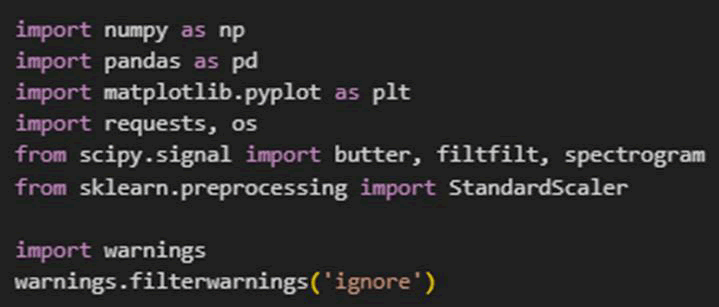
Import libraries: We import essential libraries that are essential for data handling and visualization (Figure 1).

FIG. 1. General libraries imported.

Data acquisition and setup

Setting GPS time and detector: For this study, we focus on a specific GW event (GW150914, the first confirmed observation of GWs from colliding black holes) (Figure 2) [3].

FIG. 2. Locating GPS time for Binary Black Holes merger (BBH) event GW150914 and choosing the Hanford (H1) detector.

Importing time series package

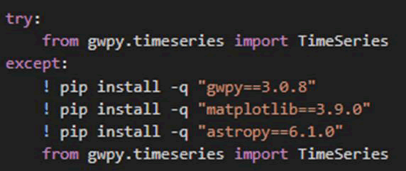
We ensure that we can successfully import time series from GWPY by installing the other required packages necessary for this installation (Figure 3) [4].

FIG. 3. Importing time series from GWPY.

Downloading and reading data

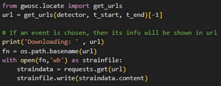
The GW data is downloaded and read into a time series object (Figure 4).

FIG. 4. Downloading and reading the GW data with the time series package imported in the last subsection.

Data extraction and handling missing values

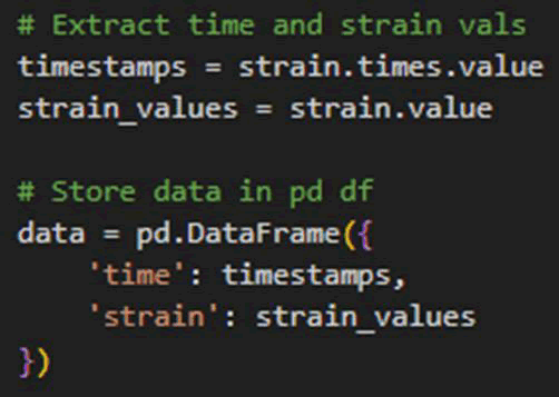
Extracting data: The timestamps and strain values are extracted and stored in a panda’s data frame (Figure 5) [5].

FIG. 5. Extracting the time and strain features from the raw GW data file.

Handling missing values

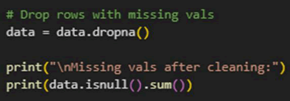
Any missing values in the dataset are dropped to ensure clean data (Figure 6).

FIG. 6. Dropping any Nan values from the dataset.

Data noise filtering and normalization

Band-pass filtering

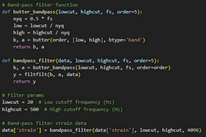
Noise filtering is crucial in GW data analysis due to the presence of various noise sources that can distract us from the true signal. One common method is band-pass filtering, which allows signals within a specific frequency range to pass through while reducing the significance of signals outside this range [6].

Purpose: The goal of band-pass filtering is to isolate the frequency range where GW signals are expected to be prominent, thus reducing the impact of noise outside the frequency ranges [7].

Application: The low cutoff frequency (20 Hz) and high cutoff frequency (500 Hz) are chosen based on the expected characteristics of a BBH event [8].

Importance: Applying a band-pass filter helps in enhancing the Signal-to-Noise Ratio (SNR) of the GW data, increasing the exposure of the actual signal (Figure 7).

FIG. 7. Butter band pass function designs a band-pass filter with specified low and high cutoff frequencies, while band pass filter function applies the designed filter to the GW data, removing noise outside the specified frequency range.

Data normalization

Normalization is another crucial preprocessing step that adjusts the GW data to a common scale, making it easier to analyze and compare [9].

Purpose: Normalization ensures that the strain data have a mean of zero and a standard deviation of one. This is particularly important for the future application of ML algorithms that are sensitive to the scale of the data [10].

Importance: Standardizing the strain data is essential for ensuring that all features contribute equally to the analysis and for improving the performance of ML models (Figure 8).

FIG.8. Standard Scaler function standardizes the features so that they’re easier for ML algorithms to analyze.

Discussion

Data inspection

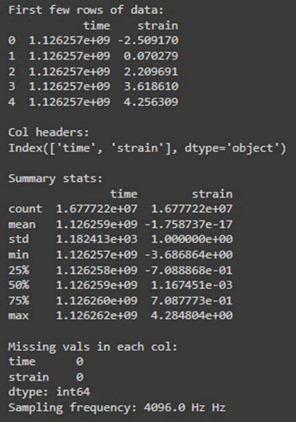
Initial data inspection: We briefly look at the data after it’s being preprocessed (Figure 9).

FIG. 9. Characteristics and features of the preprocessed GW data.

Data visualization

Visualization is a key part of data analysis, providing intuitive insights into the structure and characteristics of the GW data. Below, we explain the purpose and significance of each plot used in this section [11].

Time series plot

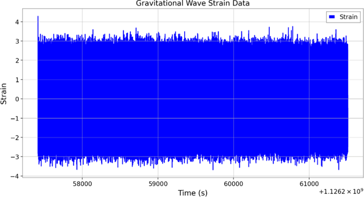
We visualize how the strain data changes over time (Figure 10).

FIG. 10. Graph of time-series plot (strain data versus time).

In the plot, peaks and troughs may correspond to significant events such as black hole mergers or neutron star collisions and it is useful for initial data inspection, allowing us to identify the presence of potential GW events [12].

Spectrogram

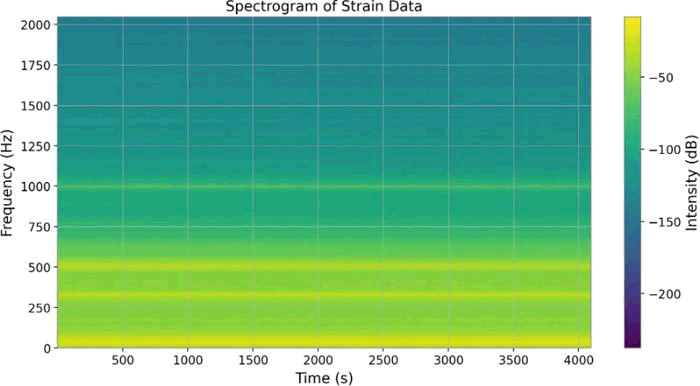
We visualize how the frequency content of the strain data changes over time (Figure 11).

FIG. 11. Graph of spectrograms (strain data’s frequency versus time).

This plot helps identify transient events and their frequency components, which are crucial for distinguishing between noises and actual GW signals. Additionally, spectrograms provide a detailed view of how the signal’s frequency content evolves and spectrogram data can be used as 2D GW data for the implementation of certain ML models [13-17].

Histogram

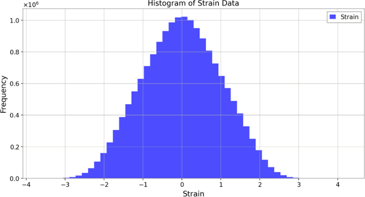
We visualize the distribution of strain values (Figure 12) [18].

FIG. 12. Graph of histogram (frequency distribution of strain data).

This plot provides an overview of the data’s spread, central tendency and outliers. This is useful for identifying any anomalies or patterns in the data. Besides this, understanding the distribution of the strain values is crucial for subsequent statistical analysis and for ensuring that the GW data meets the expectations of various ML algorithms [19,20].

Conclusion

In this paper, we have demonstrated the integration of astrophysical data analysis with programming techniques to preprocess, filter and visualize GW data. Band-pass filtering effectively reduces noise, enhancing the SNR. Normalization ensures that the data is on a standard scale, improving statistical analysis and future ML model performance. The visualizations (time-series plot, spectrogram, and histogram) provide critical insights into the GW data, enabling the plain identification of GW events and the assessment of data quality. Al-though ML is not applied in this paper, the preprocessing methods discussed are essential for preparing the data for future ML applications in GW analysis.

References

1. Abbott BP, Abbott R, Abbott T, et al. Observation of gravitational waves from a binary black hole merger. Phys Rev Lett. 2016;116(6):061102.
2. Abbott BP, Abbott R, Abbott T, et al. GW170817: Observation of gravitational waves from a binary neutron star inspiral. Phys Rev Lett. 2017;119(16):161101.

   [Google Scholar]

3. Amaro-Seoane P, Audley H, Babak S, et al. Laser interferometer space antenna. Instrum Methods Astron. 2017;1702.00786.

   [Crossref] [Google Scholar]

4. Abbott R, Abbott TD, Abraham S, et al. GWTC-2: Compact binary coalescences observed by LIGO and Virgo during the first half of the third observing run. Phys Rev X. 2021;11(2):021053.

   [Crossref] [Google Scholar]

5. Martynov DV, Hall ED, Abbott BP, et al. Sensitivity of the Advanced LIGO detectors at the beginning of gravitational wave astronomy. Phys Rev D. 2016;93(11):112004.

   [Google Scholar]

6. Fairhurst S. Source localization with an advanced gravitational wave detector network. Class Quantum Gravity. 2011;28(10):105021.

   [Google Scholar]

7. Finn LS, Chernoff DF. Observing binary inspiral in gravitational radiation: One interferometer. Phys Rev D. 1993;47(6):2198.

   [Crossref] [Google Scholar] [PubMed]

8. Abbott BP, Abbott R, Abbott T, et al. GWTC-1: A gravitational-wave transient catalog of compact binary mergers observed by LIGO and Virgo during the first and second observing runs. Phys Rev X. 2019;9(3):031040.

   [Google Scholar]

9. Schutz BF. Networks of gravitational wave detectors and three figures of merit. Class Quantum Gravity.  2011;28(12):125023.

   [Google Scholar]

10. Singer LP, Price LR, Farr B, et al. The first two years of electromagnetic follow-up with advanced LIGO and virgo. Astrophys J. 2014;795(2):105.

    [Google Scholar]

11. Abbott BP, Abbott R, Abbott TD, et al. Tests of general relativity with GW150914. Phys Rev Lett. 2016;116(22):221101.

    [Crossref] [Google Scholar] [PubMed]

12. Abbott BP, Abbott R, Abbot TD, et al. Astrophysical implications of the binary black hole merger GW150914. Astrophys J Lett. 2016;818(2): L22.

    [Google Scholar]

13. Aasi J, Abbott BP, Abbott R, et al. Advanced ligo. Class Quantum Gravity. 2015;32(7):074001.

    [Google Scholar]

14. Abbott BP, Abbott R, Abbott TD, et al. Improved analysis of GW150914 using a fully spin-precessing waveform model. Phys Rev X. 2016;6(4):041014.

    [Google Scholar]

15. Abbott R, Abbott TD, Acernese F, et al. GWTC-3: Compact binary coalescences observed by LIGO and virgo during the second part of the third observing run. Phys Rev X. 2023;13(4):041039.

    [Google Scholar]

16. Abbott BP. A gravitational-wave standard siren measurement of the Hubble constant. Nature. 2019;551(7678): 85-88.

    [Google Scholar]

17. Abbott BP. Multi-messenger observations of a binary neutron star merger. Astrophys J Lett. 2017;848: L12.

    [Google Scholar]

18. Abbott BP. Observation of gravitational waves from a binary black hole merger. Phys Rev Lett. 2016;116(6): 061102.
19. The LIGO Scientific Collaboration, the Virgo Collaboration. GWTC-1: A gravitational-wave transient catalog of compact binary mergers observed by LIGO and Virgo during the first and second observing runs. Phys Rev X. 2019;9:031040.
20. The LIGO Scientific Collaboration, the Virgo Collaboration. GWTC-3: Compact binary coalescences observed by LIGO and Virgo during the second half of the third observing run. arXiv preprint arXiv, 2021.