Short communication
, Volume: 6( 2)An Inverse Problem for a Single Orbit
- *Correspondence:
- Bozis G , Department of Physics, University of Thessaloniki, Greece, Tel: +30 2 310 998 111; EMail: gbozis@auth.gr
Received: May 30, 2018; Accepted: June 8, 2018; Published: June 15, 2018
Citation: Bozis G. An Inverse Problem for a Single Orbit. J Phys Astron. 2018; 6(2):153
Abstract
Introduction
The inverse problem of Dynamics for monoparametric families of orbits F(x,y)= c, produced in a potential field, has been studied in the past for various versions (e.g. for one or two or three parametric families, for two or three dimensional potentials in Cartesian or curvilinear coordinates, in inertial or rotating frames etc) [1].
In this report we refer to the planar motion of a unit mass material point P in an inertial frame Oxy, in a two-dimensional potential V= V(x,y), tracing one orbit (or a branch of the whole orbit) given by the equation y= f(x). We answer two questions: (a): The two functions V=V(x,y) and y=f(x) are given arbitrarily. Are they consistent? (b): An equation y= f(x) is given arbitrarily. For which potentials this equation can stand for an orbit?
Notation
We denote by Vf = Vf (x )= V(x,y=f(x)). (It stands to reason to call it orbital potential). Similarly e.g. 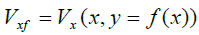 and
and 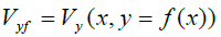 . For an arbitrary function A(x,y) we have: Af = A(x,y=f(x)). We consider A(x,y) as adequate if its orbital value is not infinity, i.e. if
  . The total energy of the point P is Ef .
Two Theorems-Examples
Theorem A
An observed branch of an orbit y= f(x) (with f”(x) ≠ 0) can be produced by a given potential V= V(x,y) if and only if
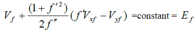 (1)
(1)
As a hint for the proof, we refer to Szebehely’s formula for monoparametric families (as modified by Bozis (1995)) with an
appropriate interpretation of the slope function γ (x, y) of the family and the help of both the orbital functions Vf(x) and the orbital function 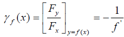 , introduced here.
Example: Let us verify that the upper branch of the Newtonian ellipse 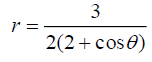 i.e.,
i.e.,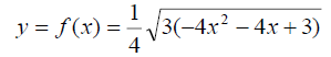 with
with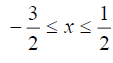 and Newton’s potential
 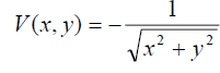 are compatible. Indeed, with e.g.
 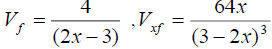 etc., the left hand side of equation (1) gives
  , as expected.
Theorem B
All potentials V(x,y) which (for adequate initial conditions, consistent with Ef ) can produce an observed branch of orbit y= f(x) are given by the formula:
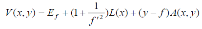 (2)
(2)
where 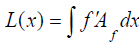 . The function A(x,y) is an adequate arbitrary function and (with the constant of the indefinite integral
L(x) taken equal to zero) Ef is the energy of P.
. The function A(x,y) is an adequate arbitrary function and (with the constant of the indefinite integral
L(x) taken equal to zero) Ef is the energy of P.
To prove the theorem B, we only need verify that, indeed, the orbit y= f(x) and the potential (2) are consistent, i.e. that they satisfy the equation (1).
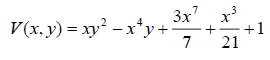
Example: For 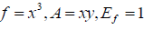 we have
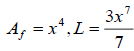 . So, formula (2) gives one out of the infinitely many
potentials which can produce the orbit y = x3 with Ef=1. For
. So, formula (2) gives one out of the infinitely many
potentials which can produce the orbit y = x3 with Ef=1. For  (so that
 ) this potential is
Comments
i. The function y=f(x) is real if Ef ≥ Vf and is defined in an interval of the x-axis which can be found from the inequality L(x) ≤ 0.
ii. If the observed (given) orbit is a straight line f (x) = λx +μ (in which case f”(x)=0), the above formulae (1) and (2) are not applicable. Then, an affirmative answer to the question 1(a) is given if Vyf = λVxf. As to the formula for the question (1b) (giving the totality of potentials producing the straight line f (x) = λx +μ ) now it reads:
 (3)
(3)
where a(x +λy),b(x, y) are arbitrary functions of their respective arguments.
It is directly shown that all the potentials (3) satisfy the relation Vyf = λVxf.