Original Article
, Volume: 5( 4)Refining Planetary Radius Calculations by Exploring the Geometry of Transit Photometry
- *Correspondence:
- Pranav AR Candidate for Bachelor of Science, Honours, Department of Physics and Astronomy, University of Waterloo, Canada
Tel: +972 1-800-660-660; E-mail: pratra16@gmail.com
Received Date: October 03, 2017 Accepted Date: November 10, 2017 Published Date: November 16, 2017
Citation: Pranav AR. Refining Planetary Radius Calculations by Exploring the Geometry of Transit Photometry. J Phys Astron. 2017;5(3):125
Abstract
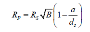
This paper has altered what appears to be the common equation taught and used to calculate the radius of an extrasolar planet, by way of transit photometry. The standard equation is: Where, RPlanet is the radius of the planet, RStar is the radius of the star and B is the percentage of light blocked by the planet during a transit, expressed as a decimal.
Where, a is the semi-major axis of the planet’s orbit (i.e. its orbital radius) and dStar is the distance from the observer to the star. There are also two additional derivations in this manuscript, which allow for calculation of the radius using angular measurements. In previous versions of this paper, author has labelled the variables in the equation differently. This is only important for those who have read or intend to read Versions 1 and 2 of this manuscript. The additional factor in the parentheses does not always make the most significant difference, considering the fraction evaluates to nearly zero in most exoplanetary cases, but it could make a difference considering other calculations depend on an accurate radius calculation, such as volume and density, for example. This aim of this equation and of this paper is to improve astronomical calculations that make use of exoplanetary transits and transit photometry. The previous, more common equation does not take into consideration the distance of the planet from its parent star. That is what this paper seeks to fix.
Keywords
Photometry; Astronomy; Star
Introduction
Studying astronomy began with discovering our home in space, our place in the vastness of the cosmos. Over time, it has gradually developed into giving humanity a deeper understanding of what the universe is made of, what laws govern it and how lucky we are to live on a planet like Earth. Situated in the middle of the habitable zone of our solar system, our home planet Earth is unique in that it has liquid water covering most of its surface, but it is also special due to its general consistency regarding temperature and the seasons. Our planet has hardly any uninhabitable places and as a result, we find life even in places we never expected to.
In recent years, however, our planet has become harsher with vast climate changes, ranging from extreme heat and cold to wild temperature swings and increasingly violent storms. This has caused the Earth to become less favourable to life, resulting in many extinctions. While most of these extinctions are due to human activity, there are some dangers to the Earth that are not the fault of humanity. Notable examples of unavoidable threats include asteroid impacts, supervolcanic eruptions (IFLScience, 2017) and the eventual superheating of the Earth due to the Sun’s growth into a red giant.
As a result, the attention to detail in astronomy has grown. The Earth is more than capable of supporting life for the time being, but greater dangers in the future, near and far, are causing us to look to the heavens for new homes once Earth is no longer suitable for life.
In order to find potentially new homes, we need to be able to know something about our target planets. That is where this paper comes in. While mass, period, radius and velocity, among other properties, of a planet are all observable or calculable, it is only the radius calculation that author will be altering in this paper.
The Development of this Paper
Author has developed the initial version of this paper to clarify the calculation methods for measuring the radius of an extrasolar planet by refining one of the many formulae used when attempting to determine useful information about an extrasolar planet. Across a number of astrophysics lectures, author and his classmates learned and used an equation that struck me as inaccurate, and, consequently, I quickly began working to develop a more precise version of that equation. In previous versions of this paper, author found that the effects of using my altered formula were significantly greater when used at smaller scales, i.e. closer to home. This document thoroughly explains the thought process behind this idea, as well as any derivations leading to the final equation.
Current Methods
Transit photometry
Transit photometry is one of the common methods scientists use today to help determine characteristics of extrasolar planets, or exoplanets. This method deals with the measurement of light intensity from a distant star, watching for a periodic drop in the intensity of light. Once we obtain the information regarding the intensity drops, a variety of other facts can be determined. In particular, we are interested in calculating the radius, volume and density of extrasolar planets, where volume and density are two calculations that depend on the calculation of the planet’s radius.
The current radius calculation
The current radius calculation involves the use of circular images of the star and its companion planet, as shown in Figure 1.

Figure 1: Planet P (grey) passes in front of Star S (white). White and black lines mark their radii, respectively. Were this image a video clip, Planet P would cross the face of Star S from one side to the other.
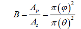
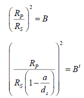
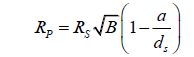
In order to calculate the radius, we use the amount of light blocked, B, by the planet as it passes in front of the star, which is equal to the area of the circular cross-section of the planet divided by the area of the star. Solving for the radius of the planet, RP, we get,
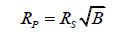
where RS is the radius of the star [1].
The issue with this calculation method is that the distance between the planet and the star is not taken into account [2]. The calculation utilizes circular projections of the star and the planet, rather than the spheres with a distance between them that they actually are.
Thus, the calculation is done as though the star and planet are two-dimensional objects, as shown in Figure 2.

Figure 2: Shown at a different angle, demonstrating the inaccuracy of the calculation, since this is not how stars and planets exist in the universe.
As seen in Figure 2 the calculation of the radius of an extrasolar planet is done under the assumption that the planet does not orbit at any distance greater than zero from its parent star.
The problem
The issue with this calculation is that planets that are farther away from their parent star are closer to us, thereby appearing larger from our viewpoint on Earth. This causes the planet to block out more of the starlight, giving us an inaccurate measurement of the radius if we use the equations described above.
The equation for calculating the radius of a planet should ideally be as accurate as possible, considering the fact that volume and thereby density calculations depend on the radius measurement.
In the following section, author will alter Figure 2 to make it more realistic, followed by modifying the equation used to calculate the radius of a planet by way of transit photometry. Note that this method can technically be used to calculate the radius of any body transiting a star, including Venus, Mercury and the Moon as they pass in front of our Sun.
Results and Discusion
Revising radius calculations
As discussed above, the issue with the present formula is that the dimension of depth is completely disregarded [3]. As shown in Figure 2, the current calculation is done under the assumption that the distance between the observer and the exoplanet is the same as the distance between the observer and the exoplanet’s parent star. However, this needs to be taken into account. As an object moves closer to an observer, it does not increase in physical size, but it does increase in angular size. The perspective we have from our planet is important to take into consideration.
During the special case of a solar eclipse, the Moon blocks out virtually all of the Sun’s light. Thus, if we were to attempt to calculate the radius of the Moon using the equation.
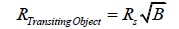
we would get a very inaccurate answer. Since most of the Sun’s light is blocked, B≈1 (since it is a percentage expressed as a decimal value), and, by extension, √B≈1.
-Then,
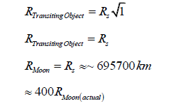
As you can see in the calculation above, usage of the dimension of depth is imperative to acquiring accurate values. This value was acquired without consideration of the third dimension and this has yielded an incredibly inaccurate answer.
In subsequent calculations, we will test the current equation and the new equation for a variety of different cases.
Deriving a new equation
We will derive a new, more accurate equation with the use of triangles. To begin, let us consider a triangle including the observer, the exoplanet and its parent star.
This can be difficult to express in words. Examine the diagram on the following page. Implications of this diagram will be discussed later on.
We will now examine the implications of Figure 3. Though very simplistic, the diagrams will be key to clearly and logically deriving a new and more accurate equation for calculating the radius of a planet using transit photometry.

Figure 3: This diagram shows the observer (eyeball on the left), an extrasolar planet (blue) and its parent star (yellow). This depiction is not to scale. Observe the diagram and you will notice that the star of diameter 2RS and a radius of RS has an angular diameter of 2θ and an angular radius of θ. Note that the exoplanet of diameter 2RP and radius RP has an angular diameter of 2φ and an angular radius of φ. dP is the distance from the observer to the extrasolar planet, while dS is the distance from the observe to the exoplanet’s parent star. While it is not shown in the diagram, the line from the observer passing through the centre of the planet and star has been approximated to be perpendicular to the lines showing the radii of the two bodies.
Implications of FIG. 3
Examine Figure 3 Notice that if we were to move the planet towards the left, i.e. closer to the observer, it would appear larger in size. However, if we moved it towards the right, i.e. closer to its parent star, it would appear smaller to the observer. The physical size remains constant, though the angular size is different and depends on the observer’s distance to the planet (Figure 4).

Figure 4: A basic visualization of the lines and angle discussed in this section.
One point to note about the use of a right angle triangle in this diagram is that the right angle is an approximation. The line that passes along the surface of the planet is a line tangent to a specific point on the surface, beyond which the planet is hidden from view to observers by its own curvature. This point and the centre point of the planet are connected by an imaginary line which makes an angle with the line that passes through the centre of the planet. This angle would be exactly 90° if 50% of the planet’s surface was visible to observers. However, this is not the case, as one can only see 50% of a sphere when positioned an infinite distance away. This is shown in the equation:
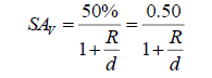
where SAV is the visible surface area of a sphere, R is the radius of the sphere and d is the distance away from the surface of the sphere an observer is [4].
As d→∞, R/d approaches zero. Thus, SAV→0.5=1/2. We have approximated the distance to a given exoplanet to be infinite. In any following images with a similar configuration, the same approximation is used unless otherwise specified.
The exact position of planet P’ is not defined in the diagram. However, its semi-major axis, a, can be determined by monitoring the system to calculate the period of the planet.
Implications of FIG. 5
Upon close observation of Figure 5, one can see that two similar right triangles are created. The smaller one is created by the planet P’, while the larger one is created by planet P. In actuality, planet P’ denotes the actual size and position 1 of planet P. Thus, it should be noted that this diagram is of a planetary system with only one planet. Planet P does not exist. However, it will be discussed as though it exists in the system, for the purpose of fully understanding the diagram.

Figure 5: A combination of the current calculation measurement from FIG. 1 and 2 and the different scenario of FIG. 3 which adds in a distance between the planet and the star. With the current calculation method, we picture the planet to be in an orbit with semi-major axis a=0, as shown by planet P overlapping its parent star. However, if we consider a semi-major axis a>0, we get the case of planet P’ (with red and orange markings).
Notice in the figure that both planets have an angular diameter of 2φ. This means that they both appear the same size from Earth and block an equal amount of their parent star’s light. Thus, these two planets are observationally identical in this manner. Therefore, if we were to use the equation that is currently applied, we would calculate the radius of both planets to be identical, since B is the same for both planets when they transit their parent star.
Notice as well that planet P cannot actually exist in this arrangement, since it has a nonexistent semi-major axis. It does not orbit its parent star; rather, it is within the star. The position and size of planet P is simply what we observe in our calculations when we neglect the dimension of depth. When we add in the third dimension, planet P is found where planet P’ is shown in the diagram; it is the same planet, but smaller and at some distance a from its parent star [2].
So, if we make use of the similar triangles that we have just created within Figure 5, we will determine a more accurate radius for the planet in this system. It cannot be overemphasized that planet P does not exist and is merely a misrepresentation of planet P’. Therefore, if we can adjust the way we look at the configuration of this planetary system by removing planet P and properly accounting for the differences between planets P and P’ in the diagram, we will actually correct the size of the planet in this planetary system. In our calculations, the final calculation will give us the size of planet P’, i.e. the actual size of planet P. To begin, let us remove some of the shapes from the image above. We will be focusing on the two similar triangles with an angle φ in one corner. This means we will be ignoring the triangle that includes a line tangent to the star, with an angle θ in one corner. The triangles we are interested in are shown below.
Determining a new equation
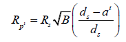
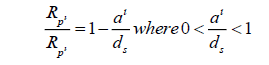
If we observe Figure 6, we can see that the true radius of the exoplanet, RP’, is related to the radius we would otherwise calculate using the current method, RP.

Figure 6: This figure represents the same configuration as FIG. 5, but it has uncluttered the image by removing the spheres and the largest triangle so that it is easy to see the similar triangles that are of interest to us.
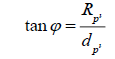
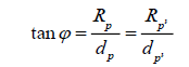
Observe the smaller triangle. Notice that,
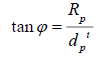
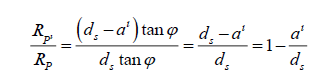
Observe the larger triangle. Notice here that,

where RP is the radius we calculate with the normal equation and d_P=d_S in this case. We will substitute in d_S for d_P and set the two equations equal to each other, since both equal tanφ.
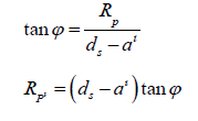
Thus, we get,

However, we also know that  Let us substitute this in as well and isolate for RP’.
Pause and observe the diagram again. Note that  We can substitute this into the equation and complete our redefinition of the radius calculation formula.
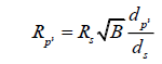
Simplifying the brackets, we get,
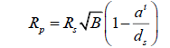
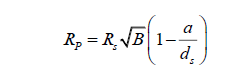
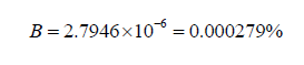
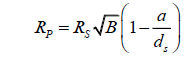
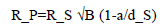
Since planet P does not exist, this equation looks exclusively at one planet. To make this clear, the equation can be expressed without apostrophes, unless described in terms of the current equation, in which case the radius values should be differentiated. That is,
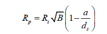
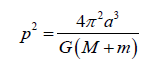
This is the final equation for calculating the radius of an extrasolar planet [2]. This is true for calculating the radius of a planet by way of transit photometry, where RS is the radius of the planet’s parent star, B is the percentage of starlight blocked by a planet expressed as a decimal, a is the planet’s semi-major axis and dS is the distance from the observer to the star. Note that a can be calculated by monitoring the period of the planet, using the formula,
Comparing the new radius with the old equation, we discover that it is slightly smaller, since the new multiplicative factor is smaller than one.
An alternate equation
Previously, we spent a lot of time discussing angular sizes before switching to physical sizes. However, angular sizes can be used to define the physical radius of a planet as well.
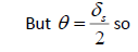
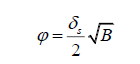
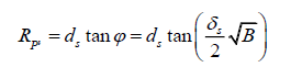
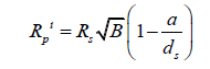
Recall that the angular diameter of the parent star, δ_S, is the same as 2θ, meaning it has an angular radius of θ. Similarly, the angular diameter of the planet, δ_P, is the same as 2φ, meaning it has an angular radius of φ. If we recalculate the original equation, we get,
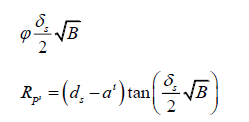
Solving for φ, we get,

If we look at the diagrams again, we will see that,
Since we are interested in solving for RP’, we will set,
We also know that,  so substituting this in, we will solve for RP’.
We can leave the equation as it is and calculate the physical radius of a planet by using its angular size, or, alternatively, we can replace φ and rewrite the equation.
We can check this against a similar formula using the original configuration. In the initial setup, dP was the same as dS. Therefore, we would have found the equation to be,
This, however, would be incorrect. We can still use it to check our equation, however,
This ratio is the same as the ratio we found on page 17, with the initial pair of equations. So, we can have confidence that this is the same.
We have now established a number of different ways to solve for the radius of an extrasolar planet. We can use these equations to compare against the original equation for calculations with specific circumstances rather than general cases.
Tests with data
We will now explore some specific cases involving bodies in our solar system being hypothetically observed transiting the Sun from a distance equivalent to a given star system. Be aware of the fact that the systems listed in the examples may not necessarily be positioned to witness such a transit in reality; we are simply using their comparatively great distance to gain some perspective with our answers.
Note that most of these calculations are limited because of the fact that we have no experimental data for how much of the Sun’s light is blocked by our own solar system’s outer planets.
Semi-major axis and other necessary data was retrieved from Wikipedia pages for each object in question. These do not need to be entirely accurate, because we simply need approximate values in order to gain meaningful perspective from our answers.
Calculations 1 through 4 have been transferred from Version 1, a more accurate method to determine the radius of an extrasolar planet by refining the use of transit photometry [3], while the fifth and sixth calculations were transferred from Version 2, refining transit photometry [3].
Example 1: Measuring the light blocked by Eris, from the Alpha Centauri System
dS will be the distance from Alpha Centauri to the Sun, in kilometres. This value comes out to about  km. RS, the radius of our Sun, is 695 700 km.
The radius of Eris is, in actuality, 1 163 km.
Eris’s orbital radius is 
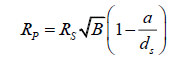
Since we have no experimental data, we will instead have to calculate the amount of light that should be blocked by Eris, using both calculation methods. So, in order to be able to use the equations described in this paper, we must rearrange for B (for the original equation) and B’ (for the revised equation) and we get,
Using the initial equation, we find that,
Using the new formula, we find that,
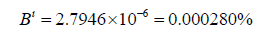
While the difference is minuscule, the second answer is more accurate because it accounts for Eris’s great distance from the Sun.
Example 2: Measuring the light blocked by 90377 Sedna, from the Alpha Centauri System
dS is about  km
km
The radius of 90377 Sedna is approximately 1027 km. This is the average of two measurements [3].
Sedna’s semi-major axis is  km.
km.
Using the initial equation, we find that,
Using the new equation, we find that,
Here, the difference between the two is larger than in the case of Eris. This is due to 90377 Sedna’s incredibly large semimajor axis. It appears that the farther away the object is from its parent star, the more this difference will assert itself. This lines up with the initial premise of the revision of the radius formula.
At this point, author would like to change our setup and begin looking closer to home. Following the same procedure as before, here are two more examples.
Example 3: Measuring the light blocked by Venus, from Earth
dS is now about 149 600 000 km, equal to 1 AU.
The radius of Venus is, in truth, about 6051.8 km.
Venus’s orbital radius is about 108 000 000 km.
Using the initial equation, we find that,
Using the revised equation, we find that,
The fact that Venus’s orbital radius is much closer in value to the total dS allowed for a relatively large change this time. The revised calculation method suggests a shadow 12.93 times larger than that predicted by the initial calculation method, which disregards the distance between Venus and the Sun. This shows that, especially within our inner solar system, it is imperative that the dimension of depth be accounted for.
Example 4: Measuring the light blocked by Mercury, from Earth
dS is now about 149 600 000 km, equal to 1 AU.
The radius of Venus is, in truth, about 2439.7 km.
Mercury’s orbital radius is about 57 909 050 km.
Using the initial formula, we find that,
Using the latter calculation method, we find that,
Because Mercury’s orbital radius is significantly smaller, the effects here are not as profound as with Venus. However, the second calculation method still predicts a Mercurian shadow 2.66 times larger than that suggested by the current formula.
Example 5: Measuring the radius of Venus using transit images
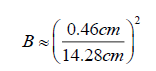
This calculation involves the use of an actual transit image. Measurements in this example were taken by measuring the sizes of the Sun and Venus across a computer screen [3], in order to find B.
RS is 695 700 km.
dS is again equal to about 149 600 000 km.
Before we continue, notice how similar this value is compared to the value we found for B’ using the modified formula in Example 3.
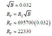
Using the original equation, we will now calculate the radius of Venus.
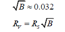
where RV is the radius of Venus, in kilometres.
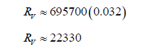
The radius of Earth is approximately 6371 km. Venus is slightly smaller, so this equation is clearly flawed. Let us attempt using the revised equation.
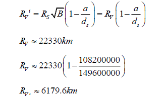
This radius value differs from the actual value by less than 128 km. The error is most probably due to inaccuracies in the ruler measurements of the digital diagram, due to the smallest increment of measurement being 1 mm.
Example 6: Calculating the radius of the Moon during an eclipse
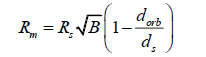
Let us attempt one final example. In this case, we will show that in the equation,
a need not be the semi-major axis of the planet. When dealing with extrasolar planets, this is the easiest value to obtain by observing the period of the planet and while it may not be entirely accurate, it will be very close if the planet’s orbit is not highly eccentric.
However, if we are dealing with a scenario where a body passes in front of a star that it is not orbiting directly, such as during an eclipse or occultation, then a is simply the distance between the transiting object and the background star.
In this simpler case, we will examine the special case of a total solar eclipse. We will approximate the amount of light blocked by the Moon to be 100% of the Sun’s light. This is not entirely accurate, as footage of totality will show that the sky is not necessarily a pitch-black dome. However, we will still use this approximation.
So, let us define what we know.
RM is the radius of the Moon, in kilometres.
The amount of light blocked is approximated to equal 100%, so B≈1.
dM is equal to approximately 384 000 km.
dS is once again equal to about 149 600 000 km.
Substituting for dorb, we get,
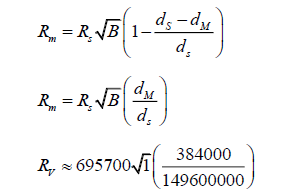
Finally, we get,
This value differs from the actual radius of the Moon by only 48.75 km.
Herefore, we can determine from this example and the examples above that this refined equation is a more accurate version than the one currently in use.
Hypothetical Examples Using Python
Explaining the code
It can be very limiting to use solely transit data acquired from telescopes, so author developed a Python program to allow a user to input a number of properties about a hypothetical planetary system and have it not only calculate the radius, but the density (another important property we look for when studying extrasolar planets) of the planet in question.
Below, author included a table of some sample calculations from this program. The columns below represent the information that the user is asked to input, as well as the information the program returns. For those who wish to test the program for themselves, see Appendix A.
Assuming there is a transit image, such as Figure 1, to use. This table assumes that the user is inputting these observational values to calculate the necessary B value for the two equations. Note that since these are hypothetical examples, the first two columns are not filled in using any such transit image.
Examine Table 1. The sample calculations have been organized such that the differences in radius and density become more and more significant progressing down the table. Notice that there is even a reasonable difference in the two radii calculations at a distance of 11 light years. While this is still relatively close to home, this shows that the equation can definitely be used in exoplanetary situations, not just examples within the solar system, as in Examples 3 through 6.
| rP* (cm) | rS* (cm) | RS (RSun) | Porb (days) | MS (MSun) | MP (MEarth) | dS (ly) | RP (km) |
RP’ (km) |
RP’/RP (%) | ρP (kg/m3) |
ρP’ (kg/m3) |
ρP’/ρP (%) |
|---|---|---|---|---|---|---|---|---|---|---|---|---|
| 0.03 | 8.9 | 0.87 | 444.3 | 0.89 | 13.4 | 4.7 | 2040.20 | 2040.19 | 99.9996 | 2249668.23 | 2249693.12 | 100.001 |
| 0.012 | 13.4 | 18.9 | 1039.2 | 24.3 | 67.8 | 7.6 | 11774.98 | 11774.83 | 99.9988 | 59207.96 | 59210.11 | 100.004 |
| 0.025 | 9.91 | 0.98 | 4454.3 | 1.1 | 0.9 | 6.1 | 1719.94 | 1719.92 | 99.9986 | 252191.47 | 252202.20 | 100.004 |
| 0.015 | 11.2 | 0.9 | 10236.8 | 0.9 | 1.2 | 5.6 | 838.57 | 838.55 | 99.9975 | 2901343.76 | 2901562.68 | 100.008 |
| 0.01 | 5.6 | 3.4 | 18091.5 | 3.2 | 31.2 | 11.3 | 4223.89 | 4223.78 | 99.9972 | 590265.10 | 590314.34 | 100.008 |
rP: radius of planet as measured in a transit image*; rS: radius of star as measured in a transit image*; RS: actual radius of star; Porb: orbital period of planet; MS: mass of star; MP: mass of planet; dS: distance to star; RP: radius of planet using the current method; RP’: radius of planet using the revised method; ρP: density of the planet using the current method; ρP’: density of the planet using the revised method
Table 1. Sample calculations comparing the current and revised equations.
Also notice that the values are close enough to the current value that they demonstrate a good accuracy compared to the current values, but it is possible to see that there are some slight differences, which, when used in the right scenarios, can make a significant impact on the calculation of the radius and density of a given planet.
Finally, notice that the slight changes in radius correlate to a larger change in the density, which can be a much more important calculation when attempting to determine the likelihood of a planet containing or consisting of liquid water. Thus, it is important to determine as accurate a radius measurement as possible, so as to not skew the calculations of volume and density [5,6,7].
Conclusion
This paper sought to refine the equation we use to calculate the radius of an extrasolar planet. This is due to the fact that we require accurate measurements to be able to determine properties of a given planet, such as density, in order to determine whether it is similar to Earth.
The main issue with the current equation is that the dimension of depth, the dimension that takes into account the displacement between a planet and its star, is completely neglected.
Through the use of diagrams, similar triangles and examples, we solidified that the adjustment factor of 1-a/d_S gives the correct equation for the radius of an extrasolar planet.
One issue about the new equation is that for planets in distant systems, a?d_S, so the adjustment factor is approximately equal to one, i.e. it hardly makes any difference. However, when used in cases such as determining the radius of a planet closer to the Sun than Earth is, the direction of depth must be taken into account.
An alternate use
Consider the following. If we find an object in our solar system passing in front of a distant star, we need to consider the dimension of depth to determine its radius based on the light blocked as it passes in front of the background star. Note that in the equation,
a does not have to be the semi-major axis of a given planet’s orbit. If we are considering a case of a body that orbits the star it is transiting, then a being the semi-major axis is the most sensible choice. However, if we were to calculate the radius of the Moon during an eclipse, as in Example 6, a would serve simply as the distance between the transiting object and the background star (in this case, the Moon and the Sun, respectively).
The importance of the calculations
The examples considered in this paper demonstrate that the revised equation makes a difference in all cases, albeit a small one for greater distances. However, if we use an incorrect radius value for an exoplanet, we will get an inaccurate volume and thus an inaccurate density. Density can be crucial as we can attempt to determine the likelihood of a planet having plentiful water supply based on its overall density. This equation seeks to reduce the errors in these calculations.
This paper was written to draw attention to need for accuracy with this equation and to provide a suitable solution. While some minute approximations were made, using the revised formula appears to be far more accurate than the current one. Additionally, this paper provided a new way to calculate the radius of a planet using angular measurements and basic geometry.
The conclusion of the derivations is that the radius we calculate with the traditional equation is too large. To correct it, we add in a multiplicative factor of 1-a/d_S. This takes into account the dimension of depth and gives a far more accurate picture of the perspective we have when viewing exoplanetary systems. This manuscript has sought to change how we view exoplanetary systems so that we can obtain the most accurate data. As science progresses, develops and changes, we too need to alter how we perceive the world around us and the universe beyond.
Appendix A
Python code
Below, the author has included the code used to generate Table 1.. This can be pasted into IDLE or a similar program that can run Python (V3.4), for a user to test the program with their own values. Documentation is provided in an attempt to make the code easier to understand. Inputting this code into Python should enable the user to enter their own values (see Table 1.) to generate their own planetary radii and densities using both calculation methods. This program has been tested many times, and, unless there is an error copying the code into Python, this program is fully functional.
Refining Transit Photometry
from math import pi, sqrt, atan# importing necessary functions from math module
# Screen Measurements – This program is designed to be used when the user views a transit image
Print ("Observe a photograph of a transit. Determine the following values and input them when prompted.")
RPscreen=float (input ("Please enter the radius of the planet as measured in an image.\nThis measurement should be in centimetres.\n"))
RSscreen=float (input ("\nPlease enter the radius of the star as measured in the same image.\nThis measurement should also be in centimetres.\n"))
# Observational Values
# radius of star in terms of radius of the Sun
RS=float (input ("\nPlease enter the radius of the star, in terms of the radius of the Sun.\n"))
# orbital period of planet in days
P=float (input ("\nPlease enter the period of the planet.\nThis measurement should be in days.\n"))
# mass of the star in terms of the mass of the Sun
M=float (input ("\nPlease enter the mass of the star, in terms of the mass of the Sun.\n"))
# mass of the planet in terms of the mass of the Earth
m=float (input ("\nPlease enter the mass of the planet, in terms of the mass of Earth.\n"))
# distance to star in light years
ds=float (input ("\nPlease enter the distance to the star.\nThis measurement should be in light years.\n"))
# Constants
G=6.67e-11
# Calculations
RS=RS*695700 # converting from RSun to km
M=M*(1.989e30) # converting from MSun to kg
m=m*(5.972e24) # converting from MEarth to kg
P=P*86400 # converting period into seconds for semi-major axis formula
dS=ds*(9.461e12) # converting distance to star into kilometres for radius formula
B=(RPscreen/RSscreen)**2 # blocked light
a=float (((G*(M+m)*(P**2))/(4*(pi**2)))**(1/3)) # semi-major axis in metres
a=a/1000 # converting a from metres to kilometres for radius calculations
# Calculating Radius – Current Method
RPcurrent=RS*(sqrt (B)) # current radius
RPitoEc=RPcurrent/6371 # radius of the planet in terms of (ito) the radius of Earth
Print ("\n\n\n\n\nUsing the current calculation method,\nthe radius of the planet is", RPcurrent, "km,\nor", RPitoEc, "times the radius of the Earth.\n")
# Calculating Radius – Revised Method
RPnew=RS*(sqrt (B))*(1-(a/dS)) # new radius
RPitoEn=RPnew/6371 # new radius of the planet in terms of (ito) the radius of Earth
Print ("\nUsing my new method,\nthe radius of the planet is,", RPnew, "km,\nor", RPitoEn, "times the radius of the Earth.\n")
# Comparing Radius Calculations
Rcompar=100*(RPnew/RPcurrent)
Print ("\nComparing the radii from the two calculations,\nmy new radius is", Rcompar, "% the size\nof the current method's value.\n\n\n")
# Calculating Density – Current Method
RPcurrent=RPcurrent*1000 # converting km to m
Vcurrent=(4/3)*pi*((RPcurrent)**3) # volume, m3
Dcurrent=m/Vcurrent # density, kg/m3
DitoH2Oc=Dcurrent/1000 # density in terms of density of water
Print ("\nUsing the current calculation method,\nthe density of the planet is", Dcurrent, "kilograms per cubic metre,\nor",DitoH2Oc, "times the density of water.\n")
# Calculating Radius – Revised Method
RPnew=RPnew*1000 # converting km to m
Vnew=(4/3)*pi*((RPnew)**3) # volume, m3
Dnew=m/Vnew # density, kg/m3
DitoH2On=Dnew/1000 # density in terms of density of water
Print ("\nUsing my new calculation method, the density of the planet is", Dnew, "kilograms per cubic metre,\nor", DitoH2On, "times the density of water.\n")
# Comparing Density Calculations
Dcompar=100*(Dnew/Dcurrent)
Print ("\nSimilarly, comparing the densities from the two calculations,\nmy new density is", Dcompar, "% the value\nof the current method's value.\n").
Acknowledgements
This paper would not have been possible were it not for the instruction of material and revisions of Versions 1.1 and 2.4 by Dr. R. J. Epp, physicist and lecturer at the University of Waterloo. Dr. Epp’s lectures about exoplanets and transit photometry sparked the development of the ideas in this paper. His reviews of Versions 1.1 and 2.4 of this paper were imperative to the development of this edition. I would also like to extend my gratitude to B. Ratra, who read Version 1.2 and A. Ratra, who studied the formulae in Version 2.4, for both reviewing and offering feedback. Additionally, I would like to thank S. Ratra for reading and offering feedback on Version 1.1, regarding the clarity of the manuscript. I offer my thanks to A. Ratra for establishing contact with B. Ratra.
Additionally, I would like to thank T. Miller for reviewing the derivations used in Version 2.4.
I received a large number of assessments and diverse feedback regarding format and diction of past manuscripts, as well as a number of reviews about the calculations and I thank all who contributed. The suggestions of those who proofread all or part of the paper were taken into consideration regarding the clarity of subsequent manuscripts.
Additional thanks to
L. Blagodatskikh, A. Chandra, L. Cooper, W. Kabir, V. Ratra and I. Robinson for offering a tremendous amount of support and encouragement during the writing process of Versions 1 and 2.
References
- Epp RJ. Introduction to the Universe. Uni of Waterloo. PHYS. 2017; 175.
- Ratra PA. Refining transit photometry. 2017. Waterloo ON.
- Ratra PA. A more accurate method to determine the radius of an extrasolar planet by refining the use of transit photometry. 2017.Waterloo ON.
- Baird CS. Since one satellite can see half of the earth. why do we need more than two satellites in a given network? 2017;28.
- [No authors listed]. Angular Diameter. 2017;27.
- [No authors listed]. Wolfram Alpha: Computational Knowledge Engine (nd). 2017;30.
- [No authors listed]. Is the Yellowstone Supervolcano About to Erupt. IFLScience (nd). 2017.