Mini Review
, Volume: 12( 11)Reanalysis of the Schwarzschild Radius
Received date: Nov-22-2024, Manuscript No. tspa-24-154210; Editor assigned: Nov-25-2024, Pre-QC No. tspa-24-154210 (PQ); Reviewed: Nov-28-2024, QC No. tspa-24-154210 (Q); Revised: Dec-01-2024, Manuscript No. tspa-24-154210 (R); Published: Dec-27-2024, DOI. 10.37532/2320-6756.2024.12(12).345
Citation: Fowler J.C. Reanalysis of the Schwarzschild Radius. J Phys Astron. 2024;12(12):345.
Abstract
The Schwarzschild solution to Einstein’s field equations reveals a potential singularity at a critical point known as the Schwarzschild radius. The singularity can be eliminated by transforming to any of several alternate coordinate systems. This fact supports the current interpretation that the Schwarzschild radius poses no obstruction to the formation of black holes or the smooth motion of bodies falling freely across it. However, while it is almost universally acknowledged, this interpretation harbors inconsistencies and unresolved issues. Over the past twenty years, I have performed a thorough reanalysis of this topic in search of a resolution to these unresolved issues. In the process, I have discovered that while the mathematical analysis is correct, the current interpretation of that analysis is faulty. In its place, I propose a far more intuitive interpretation of Schwarzschild geometry that is consistent with the mathematical analysis and reconciles perfectly with all related physical observations. This new model does, however, yield predictions concerning black hole theory that differ significantly from those of the current theory.
Keywords
Schwarzschild solution; Schwarzschild geometry; Schwarzschild radius; Black holes; Event horizon
Introduction
In 1915, Einstein published his field equations for General Relativity (GR). According to his theory, the combination of matter and energy distributed within a physical region produces warpage or curvature of spacetime. Falling bodies are constrained to follow geodesics within this curved spacetime continuum. Thus, the equations of motion are determined by deriving geodesics from the corresponding metric equations, rather than by applying Newtonian methods involving force and acceleration.
The GR field equations are inherently complex; however, exact solutions have been found for some highly symmetric distributions. The first and perhaps the most well-known of these solutions was derived by Karl Schwarzschild in 1916. He confined his work to mass distributions that were spherically symmetric, neutrally charged, and non-rotating. He was able to quickly derive an exact solution for the region of empty space external to this configuration. Shortly thereafter, he followed with an idealized solution for the interior region. Tragically, Schwarzschild’s remarkable productivity halted four months later when he died of an illness contracted on the Russian front [1].
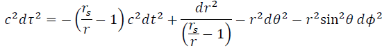
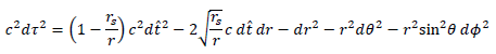
The Schwarzschild metric, which is his solution for the external region, is presented below without proof [2].

The Schwarzschild radius rs is defined as follows.

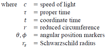
where G = Newtonian constant of gravitation
M = mass of the spherically symmetric body
The Schwarzschild metric is the primary basis for the topics and discussions presented throughout this document1. From it, geodesics can be derived that lead directly to equations of motion for free-falling or orbiting bodies2. These results have been successfully employed to predict the precession of the orbit of Mercury and the deflection of starlight as it passes near the sun [3].
Despite the amazingly successful application of these methods, there is one potentially troubling aspect of the Schwarzschild metric. A singularity occurs when r = rs. The first term goes to zero, while the second term goes to infinity. However, this singularity can be eliminated by transformation to any of several alternate coordinate systems. This implies that the singularity is strictly mathematical in nature and leads to the conclusion that the metric characterizes a perfectly smooth pseudo-Riemannian manifold [4].
Arguably, the most significant prediction of GR is that of black holes. According to the current theory, if a star’s radius is less than or equal to rs, light is red-shifted to an infinite wavelength, and the star becomes invisible to external observers. The spherical surface at r = rs is known as the event horizon and represents a point of no return. Supposedly anything that falls within the event horizon, including material objects and light itself, is unable to escape [4].
One of the best ways to understand the significance and nature of the Schwarzschild radius is to analyze the theoretical behavior of a small test body or probe released to fall freely toward it. Such analysis can be performed from either of two perspectives: one with respect to a fixed observer, and the other with respect to an observer moving in synchrony with the probe. I shall refer to the former as the fixed perspective and the latter as the onboard perspective.
The curious thing is that analysis of these two perspectives appears to yield two different outcomes. The fixed perspective predicts that the probe will approach the Schwarzschild radius asymptotically and never actually cross it. On the other hand, the onboard perspective predicts that the probe will pass smoothly across the critical radius unobstructed.
These outcomes are diametrically opposed. They cannot both be true. While there are multiple ways to analyze a probe’s motion, there is only one physical reality. In GR, motion is represented as a set of events. Those events can be tracked from any perspective using any desired coordinate system. But, while the coordinate values may differ depending on the perspective, the tracked events must be the same. The probe either crosses the Schwarzschild radius or it does not. We cannot have it both ways.
1It is assumed that the reader has some familiarity with the Schwarzschild metric. For those who desire more detailed information on its derivation and underlying theoretical principles, several excellent resources are identified in References.
2See Appendices A and B for the full derivations.
The current theory rests in favor of the onboard perspective. This is primarily justified by the fact that the onboard analysis suggests that there is a smooth, continuous geodesic from any point in the manifold to the origin. Because falling bodies follow geodesics in spacetime, it is logical to conclude that the motion of the probe must be smooth and uninterrupted as well.
This argument seems compelling, if not irrefutable. However, after twenty years of research, I have finally discovered that it is the interpretation of the onboard perspective that is in error and that the fixed perspective is correct after all. This misinterpretation has significant ramifications, and correcting it will mean rethinking many of the time-honored conclusions of GR, including the plausibility of black holes.
Analytic Preliminaries
To correct the misinterpretation of the onboard perspective, it is first necessary to perform some preliminary analysis, including a review of the basic constraints of GR theory itself.
General relativity basics
In 1905, Einstein published his formulation of what we now call the Theory of Special Relativity (SR). This theory quantifies the rules governing the motion and behavior of material objects in a flat spacetime environment, that is, one free of gravitational influence. The keystone of SR is the Lorentz transformation, which defines the relationship between the space and time coordinates of two frames of reference, S and S′, moving at a constant velocity v relative to each other [5].
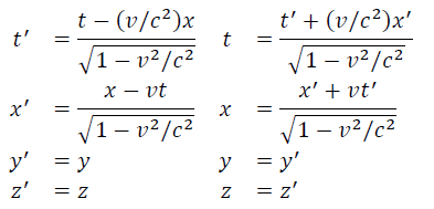
Given the occurrence of any two spacetime events E1(t1,x1,y1,z1) and E2(t2,x2,y2,z2), it is straightforward to apply the Lorentz transformation to derive the following invariant relationship, known as a spacetime interval3.

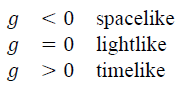
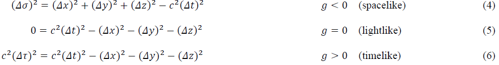
Any spacetime interval is classified into one of three categories depending on its sign. Because g is invariant, its classification is also. In other words, the classification of a spacetime interval is an intrinsic property, independent of the frame of reference.
For any spacelike interval, one can always transform to a frame of reference where the events occur at the same time but at different locations. Setting Δt =0 in equation (3) yields the following relationship.
3Throughout the document I use the (+,−,−,−) convention where the time component is positive and the space components are negative, as opposed to the (−,+,+,+) convention where the opposite is true. The choice of conventions is a matter of preference, being equivalent as long as one reverses the polarity of all corresponding relationships.
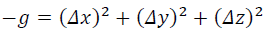
It is clear that −g represents the square of the physical distance between two simultaneous, spacelike events. This value is defined as the proper distance interval and is usually expressed using the symbol σ. Using this definition, equation (3) can be expressed as follows, emphasizing that it is valid only for spacelike intervals.

For any timelike interval, one can always transform to a frame of reference where the events occur at the same location but at different times. Setting Δx =Δy =Δz =0 in equation (3) yields the following relationship.
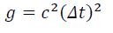
It is clear that g/c2 represents the square of the time interval between two timelike events that occur at the same location. This value is defined as the proper time interval and is usually expressed using the symbol τ. Using this definition, equation (3) can be expressed as follows, emphasizing that it is valid only for timelike intervals.

Lightlike intervals take on the following form.
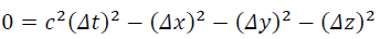
The interpretation here is that the time difference between the events exactly matches the time required for a light signal to travel between them. From the perspective of an observer moving at the speed of light, the two events occur at the same place and at the same time. In other words, the two events appear to be the same event.
The relationship between spacetime intervals can be summarized as follows:
In SR, one tracks the motion of material objects as a continuous series of events by extending equation (6) into the form of infinitesimals.

This expression defines the line element, or in SR jargon, the world line of a body with proper time τ as its invariant parameter.
Note that only the timelike relationship of equation (6) is suitable for this purpose because it is only then that all observers agree on the time sequence of events. This is a critical point that will be referenced frequently. Unless all observers agree on the time sequence of events, it is impossible to establish causality between them. In other words, one cannot determine when one event causes another unless one can establish which of the events occurred first [6].
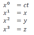
In 1908 Hermann Minkowski proposed combining time with the three spatial dimensions to form a blended entity called spacetime [7]. Accordingly, he developed a four-dimensional, geometric model for SR. To see how this works, first define coordinates in terms of the space and time variables.
Next, define the Lorentz metric as a second-rank tensor.
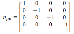
This enables equation (7) to be expressed as the metric equation for a simple, four-dimensional pseudo-Riemannian manifold, which defines what is known as Minkowski space.
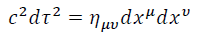
Because ημν is constant everywhere, the manifold is flat and thus models SR where the environment is free of gravitational influence.
GR extends this idea to include gravitational effects by employing variable metric components.

The components gμν are functions of xμ and are determined from the distribution of mass and energy. Thus, this metric equation models the curvature of spacetime in the form of a pseudo-Riemannian manifold.
A defining property of Riemannian manifolds is that they are locally flat. At any point, one can transform to what are known as geodesic coordinates, which satisfy the following conditions when evaluated at the point of reference:
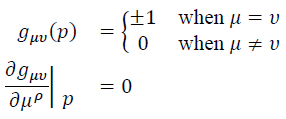
Thus, at the point of reference, the metric evaluates to a diagonal matrix of ±1 components. Such a metric characterizes a flat, local space that is Euclidean if all the components are positive, or pseudo-Euclidean if some of them are negative. Minkowski space is clearly pseudo-Euclidean.
It is this feature of Riemannian manifolds that enables Einstein’s intuitive ideas of GR to be expressed as a geometric model. For any given mass and energy distribution, spacetime events can be recorded at large as points in a pseudo-Riemannian manifold. They can then be analyzed locally in flat geodesic coordinates by applying the principles of SR. The effect of this model is to eliminate the SR restriction that the relative velocity between frames of reference must be constant. The principles of SR are applicable to all inertial frames of reference, even though they may be accelerating relative to each other, as is the case in gravitational fields.
General Relativity Constraints
For this model to work, the locally flat space must be Minkowski space. In other words, it is essential for the metric of the geodesic coordinates at any point to be precisely equal to the Lorentz metric ημν. Otherwise, it is impossible to perform SR analysis. This requirement naturally leads to certain important constraints that must be enforced to ensure the validity of the model.
The combination of ±1 metric components of the geodesic coordinate system constitutes the signature of the manifold. This is expressed as (p,q), where p is the number of positive components, and q is the number of negative components [8]. It can be shown that this signature is invariant, meaning that the values of p and q are the same everywhere within the manifold [9].
Manifolds are classified according to their signatures. A manifold with a signature of (p,0), where all the components are +1, is known as a Riemannian manifold. When p>0 and q>0, the manifold is pseudo-Riemannian or semi-Riemannian. A Lorentz manifold is a pseudo-Riemannian manifold with a specific signature of (1,3), and it is evident that any space applicable to GR must be a Lorentz manifold. It is only then that the corresponding local pseudo-Euclidean result can equate to Minkowski space.
Although this requirement is necessary, it is not sufficient. Just because equation (8) characterizes a Lorentz manifold does not mean that every point within the manifold qualifies for GR analysis. There is a second, critical constraint for the geometric model which has previously been overlooked, ignored, and/or misunderstood.
As noted earlier, the manifold signature (p,q) is invariant. However, this does not imply that the order of the ±1 components along the local diagonal metrics is. Indeed, a Lorentz manifold may include regions where any of the four diagonal elements is positive while the others are negative. From a mathematical perspective, regions with any of these possibilities may be part of the same Lorentz manifold, as long as it is nondegenerate. All one needs to show is that the determinant of the metric equation is nonzero and thus invertible everywhere. The order of local diagonal elements may vary from one region to another.
However, the only case applicable for GR analysis is the one that precisely matches the Lorentz metric ημν, being the one where the time component is positive. All others must be disregarded and rejected outright, not because of mathematical limitations, but because they violate the basic premise of GR that it must be possible to perform SR analysis locally at any point. This is only possible in Minkowski space where the time component is positive.
This restriction can be understood in another way by a closer examination of equation (8), which is the GR equivalent of equation (7). Recall the earlier point that equation (7) is only valid for timelike intervals, meaning that the right side of the equation must be greater than zero, and the time component must be positive. The same restriction applies to equation (8).
Recall that proper time is derived in SR by setting all distance intervals to zero. The same technique applies to GR. First, expand equation (8) to its full meaning.
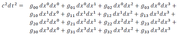
Then set all the distance infinitesimals to zero.
This is the GR definition of proper time τ. Note that this generalization is entirely consistent with the definition of proper time in SR where g00=1. In either case, proper time is the invariant parameter that quantifies the motion of material objects through the spacetime continuum.
For this to work, the value of τ must be real and nonzero, which means that g00 must be positive. This restriction is equivalent to requiring that the local geodesic coordinate systems equate to Minkowski space where the time component is positive.
Lorentz manifolds in general admit regions where g00>0, g00=0, or g00<0; which can be classified as timelike, lightlike, or spacelike respectively [10]. Relativistic analysis must be limited to timelike regions because proper time is undefined everywhere else. We say that timelike regions are time-orientable. It is only there that all observers agree on which of two events occurs first from a time perspective. In summary, valid GR analysis must be constrained by the following two principles:
• All spacetime events must be represented as points within a Lorentz manifold.
• All analysis must be restricted to timelike regions where g00>0.
Rotating frame of reference
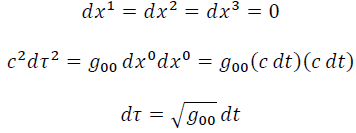
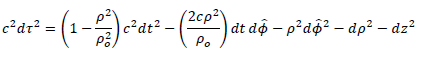
To illustrate these concepts, consider the example of a rotating frame of reference. Begin with equation (7) and transform to cylindrical polar coordinates.
Transform to a frame of reference that rotates about the z axis at constant angular velocity ω.

Define a new constant ρ0.
Eliminate the off-diagonal dtdφ̂ term by transforming to the time coordinate t̂ as defined below:
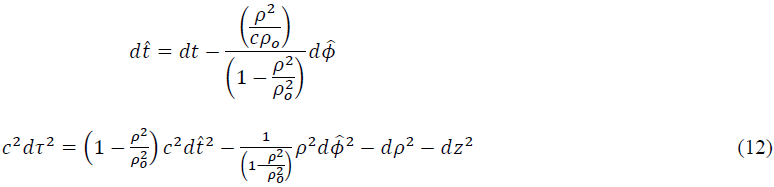
The determinant of this expression is −c2ρ2, and because its value is nonzero everywhere except when ρ=0, the manifold is nondegenerate, and thus qualifies as a pseudo-Riemannian manifold. Equation (12) can now be normalized and brought into full canonical form at ρ=a by transforming to coordinates ta and φa as defined below:
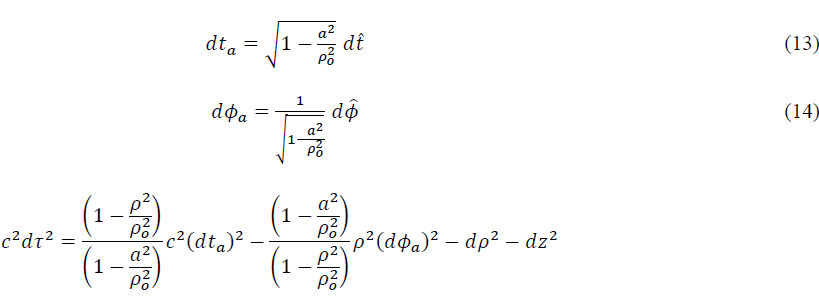
When ρ=a, this evaluates to the following form.

Note that this form exactly mirrors that of equation (9), demonstrating that coordinates ta, φa, ρ, and z qualify as geodesic coordinates at ρ=a. Because the signature is (1,3) the manifold itself is a Lorentz manifold. Because the metric is precisely the Lorentz metric ημν, equation (12) qualifies as the world line for material objects. For example, it can be used to derive timelike geodesics parameterized by τ, which describe the motion of such objects in the absence of external forces.
However, as described in the previous section, there is an important restriction. The geometric model for GR only applies when g00>0 or, in this particular case, when (1−ρ2/ρ02)>0 or equivalently when ρ<ρ0. To illustrate why this restriction exists, repeat the analysis for the case in which ρ>ρ0. In this case it is more appropriate to express equation (12) in the following form:

This time transforming to ta and φa as defined by equations (13) and (14) does not work because they assume imaginary values when a>ρ0. Instead, it is necessary to use the following definitions.
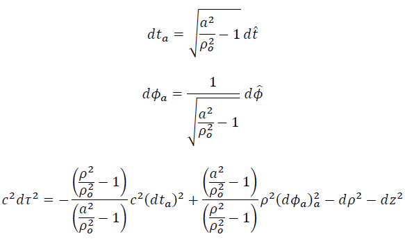
When ρ=a, this evaluates to the following form.

Again coordinates ta, φa, ρ, and z qualify as geodesic coordinates at ρ=a, but this time the metric is wrong. The signature is still (1,3), but the local space is not Minkowski space. Thus, the geometric model for GR is no longer valid. In addition, because g00<0, proper time τ assumes an imaginary value and is therefore undefined. To correct this issue it is necessary to parameterize equation (15) with proper distance σ instead of proper time τ.
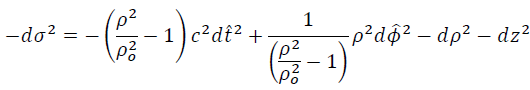
Mathematical analysis of this expression is possible; however, it is essentially worthless. For example, geodesics can be derived, but they are spacelike geodesics that provide no information regarding the time dependency of motion.
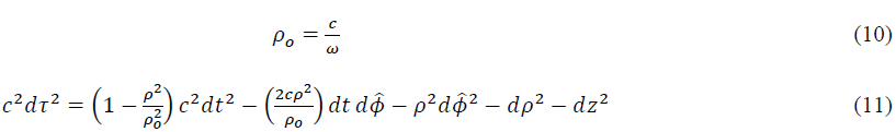
To obtain a clearer understanding of why the GR geometric model is limited to timelike regions, refer back to equation (10).

Note that ρ0ω is the velocity of a point in the rotating frame which is ρ0 units from the origin. Therefore, points in the rotating frame where ρ≥ρ0 equate to velocities v≥c. Thus, lightlike and spacelike regions correspond to frames of reference that are moving at or beyond the speed of light.
Recall that the Lorentz transformation is applicable only when v<c. This is a critical restriction that must be adhered to at all times. Everything in relativity, including all aspects of GR, is based on, and ultimately derives from, the Lorentz transformation. Thus, there are no circumstances under which relativity can tell us anything about frames of reference that are moving at or beyond the speed of light. This is a fundamental restriction that cannot be disregarded, regardless of how creative one’s imagination may be or how desperately one wishes to believe otherwise.
To summarize this rotating frame of reference illustration, the manifold characterized by metric equation (12) is a Lorentz manifold that consists of three regions identified below. These classifications are analogous to those of spacetime intervals as per equations (4), (5), and (6).
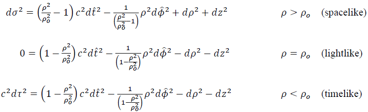
Geodesics can be derived for spacelike regions, but they must be parameterized by proper distance σ, which means that the results do not provide information about the time dependency of motion within that region. In lightlike regions, no geodesic solutions are possible because there is no invariant parameter available for that purpose.
It is only in timelike regions that proper time is defined as real and nonzero. Only then can geodesics be derived using proper time τ as the invariant parameter. These timelike geodesics are the world lines for material objects as they move through the spacetime continuum, and for that reason, GR analysis is limited to timelike regions. Material objects move along timelike geodesics. Light moves along null geodesics. Nothing moves along spacelike geodesics because, to do so, they must be moving at speeds greater than that of light.
Schwarzschild Geometry
Focus now on the spacetime manifold characterized by the Schwarzschild metric equation (1).

The determinant of this expression is −c2r4sin2θ. Because its value is nonzero everywhere except when r=0, the manifold is nondegenerate and thus qualifies as a pseudo-Riemannian manifold. The apparent singularity at r = rs can be eliminated by transformation to any of several alternate coordinate systems4.
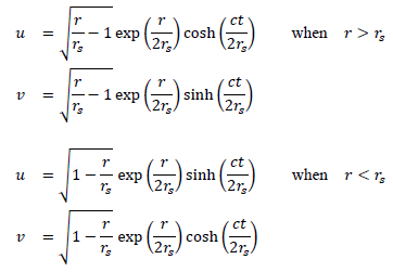
Consider the case in which r > rs. Transform to coordinates ta and ra as defined below:
Evaluate this expression at r=a.

4See Appendix C for an example of such a transformation to Gullstrand–Painlevé coordinates.
This result is locally flat, demonstrating that coordinates ta, ra, θ, and φ qualify as geodesic coordinates at r=a. Because the signature is (1,3) the manifold itself is a Lorentz manifold, and because the metric is the Lorentz metric ημν, the local space is Minkowski space. As expected, r > rs is a timelike region that fully qualifies for GR analysis.
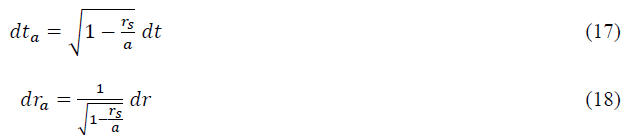
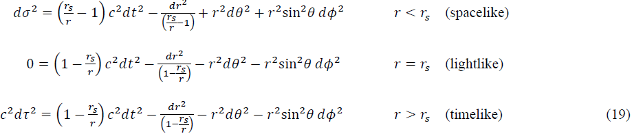
Next, consider the case where r < rs. Note that in this region the signs of the first two terms in equation (16) are reversed, so it is more appropriate to express the metric equation this way.
This time, transforming to ta and ra as defined by equations (17) and (18) does not work because they assume imaginary values when r < rs. Instead, it is necessary to use the following definitions.
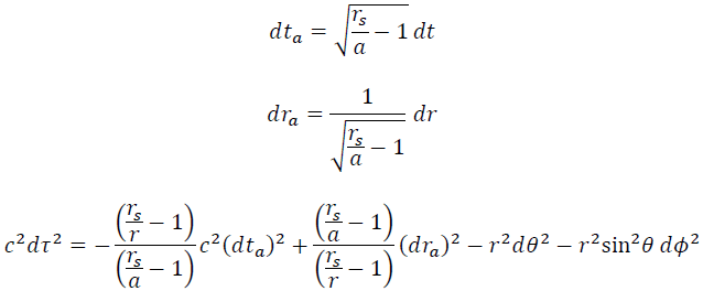
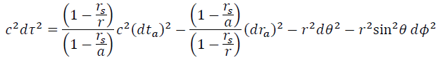
Evaluate this expression at r=a.

Again, the local space at r=a is flat, confirming that coordinates ta, ra, θ, and φ qualify as geodesic coordinates. However, this time, although the signature is still (1,3), the local metric is not the Lorentz metric ημν.
Similar to the rotating frame of reference example, the Schwarzschild metric characterizes a Lorentz manifold that includes three regions.
Surely the parallel with the rotating frame of reference is self-evident. The spacelike and lightlike regions of Schwarzschild geometry are disqualified from GR analysis in the same way as those of the rotating frame of reference and for the same reasons. It is only when r > rs that g00>0 and proper time is both real and nonzero. GR theory provides no information about time-dependent motion where r≤rs, and therefore any attempts to apply GR analysis in these regions must be summarily abandoned and disregarded. Unfortunately, despite this clear and simple conclusion, theorists have for decades felt compelled to manufacture convoluted explanations for how the application of GR theory might extend to these irrelevant regions.
The typical explanation goes something like this. When r becomes less than rs, the value of the metric goes negative, and the signs of g00 and g11 switch. This means that paths along the t axis (r, θ, φ constant) are spacelike, while paths along the r axis (t, θ, φ constant) are timelike. This suggests that the roles of coordinates r and t switch, meaning that somehow r should be interpreted as the time marker, and t should be interpreted as the radial marker. In this context, the metric’s value is positive only if dr2≠0, which means in turn that the value of r cannot remain fixed. A falling object must inevitably fall into a singularity at the center of the black hole [4]. This interpretation is a great example of the kind of mental gymnastics that become necessary when one assumes the principles of GR in regions where they simply do not apply.
So why is the disqualification of spacelike and lightlike regions so obvious for a rotating frame of reference and not for Schwarzschild geometry? In the former case, it is clear that those regions correspond to physical conditions which are known to be impossible. Relativity applies only to frames of reference moving at relative speeds slower than that of light. Thus, it is only the timelike region that corresponds to physical reality. On the other hand, it is not intuitively obvious that regions in Schwarzschild geometry where r≤rs are likewise beyond the realm of physical reality.
Attempts to apply GR analysis to points on or inside an event horizon are predicated on the assumption that the existence of black holes is, at least in principle, actually possible. On the other hand, if it can be shown that the formation of black holes is fundamentally impossible, then the entire exercise becomes pointless. If black holes are not possible, then points on or inside an event horizon do not correspond to physical reality, and thus there is no need to analyze them. To explore that idea, it is advantageous to thoroughly analyze the theoretical behavior of a small free-falling probe as it nears the event horizon.
Reconciling the Free-Falling Probe Perspectives
As briefly described in the Introduction, the behavior of a falling probe can be analyzed from two different perspectives: the fixed perspective and the onboard perspective. In this section, the topic is reanalyzed in detail to correct the misinterpretation of the onboard perspective and establish a clear reconciliation with the fixed perspective.
Fixed perspective
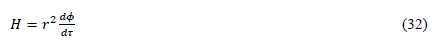
An external observer at a fixed location tracks the motion of a free-falling probe in terms of coordinate time t. Thus, the appropriate equations of motion are (35) and (36), as derived in Appendix A.
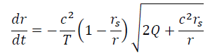
At t=0, the probe is released directly toward the black hole from point r=a with an initial local velocity va. Releasing the probe in a direct line toward the black hole equates to the initial condition dφ /dt =0, thus H=0.
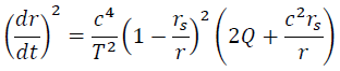
Take the square root of both sides and choose the negative sign for the inward path.

Use equation (33) to eliminate T.
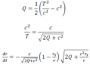
Separate the variables.
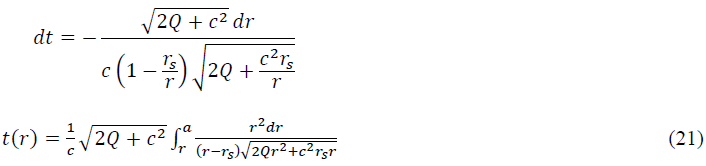
By making use of the following relationship
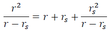
equation (21) can be expressed as follows.
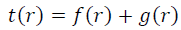

Similar to the Newtonian solution, f(r) assumes one of three forms, depending on the value of Q.

In contrast, g(r) assumes a single form for all values of Q. There is no parallel in the Newtonian solution.
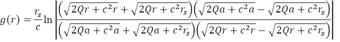
All three forms of f(r) behave well throughout the domain a≥r≥0, that is no singularities arise. However, this is not the case for g(r). Here, the expression approaches infinity as r approaches rs. Thus, for all values of Q, coordinate time t approaches infinity as well. This implies that the probe never reaches the event horizon.
For simplicity, most authors illustrate this point by presenting only the case in which Q=0. Although the math is more involved, I have chosen to include the analysis for all cases to demonstrate that the result is quite general. From the perspective of any fixed observer, the probe will not reach the event horizon in a finite period, regardless of when or where it is released or how fast it is initially moving. This result is illustrated graphically in FIG. 1.

Figure 1: Probe’s motion from the fixed perspective.
Fixed local perspective
One result of this fixed perspective is that dφ /dt approaches zero as r approaches rs. This is immediately apparent in equation (20).
It is sometimes said that the fixed perspective predicts that the probe will “freeze” near the event horizon. This concept is not intuitive and is extremely misleading.
It is important to understand that Schwarzschild coordinates r and t are ephemeris coordinates, meaning that they are simply markers or bookkeeping units used to record and catalog events. As such they do not equate to what observers actually measure, except in the special cases where the point of reference is far removed from the origin or the mass is relatively small.
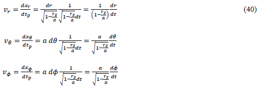
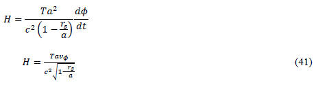
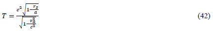
One obtains a better sense of what is going on by examining the probe’s velocity from the perspective of actual measurements taken locally by fixed observers positioned along the path. This information is readily available from equation (42) in Appendix B.
This expression establishes the value of T from the initial conditions r=a and v=va, where the initial position and velocity of the probe are measured locally at that point. However, because T is constant, the relationship holds for all values of r and vr anywhere along the probe’s path.
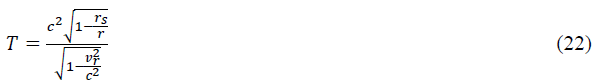
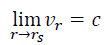
Solve this expression for vr.
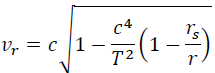
This is the probe’s velocity measured locally by a fixed observer at location r. One simply imagines an infinite set of fixed observers positioned along the probe’s path, each measuring the probe’s velocity in the same manner as it passes by. Clearly, the probe does not slow down or stop. Instead, its velocity continues to accelerate indefinitely along the entire path and approaches the speed of light as r approaches rs.
Additional insight is gained by examining the energy of the probe as it moves along the path. To do so simply rearrange equation (22) into the following form, where m0 is the rest mass of the probe.
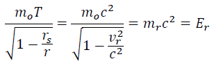
This is the expression for the total relativistic energy of the probe, measured locally as a function of its location r. It is clear that energy increases as the value of r decreases. This makes sense because it is falling through an ever-increasing gravitational potential. It is gaining energy throughout the process. It is also apparent that the energy approaches infinity as r approaches rs.
These results provide a much clearer and more intuitive understanding of why a falling probe can never reach the event horizon. Any SR aficionado knows that boosting a material object to the speed of light requires infinite energy, and is therefore fundamentally impossible. The same limitation exists for falling probes. Under no circumstances will the local conditions of spacetime curvature allow a falling probe to achieve the speed of light.
Traditional analysis of the onboard perspective
While the fixed perspective provides a clear picture of the motion of a falling probe, the onboard analysis paints an entirely different picture. The onboard observer records the motion of the probe as a succession of events occurring at the same location. Thus, the analysis must be repeated using proper time τ instead of coordinate time t. The appropriate equations of motion for this purpose are equations (32) and (34) as derived in Appendix A.
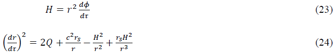
At τ=0, the probe is released directly toward the black hole from point r=a with an initial local velocity va. Releasing the probe in a direct line toward the black hole equates to the initial condition dφ /dτ =0, thus H=0.

Take the square root of both sides, choose the negative sign for the inward path, and separate the variables.
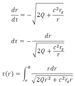
Similar to the Newtonian solution, τ(r) assumes one of three forms, depending on the value of Q.
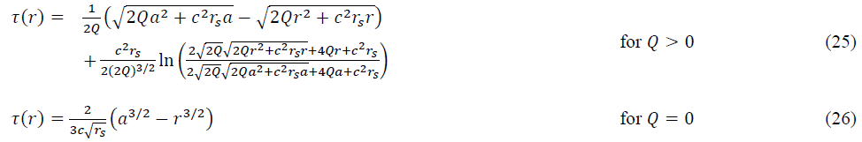

All three forms behave well throughout the domain a≥r≥0. Unlike coordinate time t measured by the fixed observer, proper time τ measured by the onboard observer does not diverge to infinity anywhere along the path. This simple fact is the most compelling and seemingly irrefutable evidence that the probe will fall smoothly across the event horizon. Because there appears to be a smooth geodesic connecting the point of release all the way to the center of the black hole, it seems reasonable that the motion of the falling probe must also be smooth and uninterrupted. This interpretation is illustrated graphically in FIG. 2.

Figure 2: Probe’s motion from the onboard perspective.
Corrected analysis of the onboard perspective
The traditional analysis of the onboard perspective, as presented in the prior section, seems intuitively correct. However, while the mathematical analysis is correct, the corresponding interpretation is not. In this section, I correct the interpretation with a new model that reconciles perfectly with that of the fixed perspective.
The key to correctly interpreting the onboard perspective is that equations (23) and (24) are valid only when r > rs. Recall that proper time τ is defined only in this exterior region, and any relationships that depend on τ cannot be applicable anywhere else. Timelike geodesics parameterized by proper time τ are only possible where r > rs. When r < rs, geodesics must be parameterized by proper distance σ, and are therefore spacelike. Thus, what appear to be smooth paths from r=a to r=0 are really composite paths made up of timelike geodesics where r > rs, joined with spacelike geodesics where r < rs. In FIG. 2, timelike geodesics are depicted in blue, while spacelike geodesics are depicted in red.
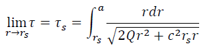
Spacelike geodesics do not depend in any way on proper time τ. Therefore, while equations (25), (26), and (27) are correct, they only apply when r > rs and cannot be the basis for conclusions applicable to any other region5. They certainly don’t tell us that the probe crosses the event horizon. What these equations tell us, and ALL they tell us, is that proper time τ, measured by the onboard observer, approaches the finite value τs defined below, as the probe approaches r = rs.
5Incidentally since equation (1) is valid only when r > rs ,as per equation (19), the same restriction applies to everything derived in Appendix A.
5Incidentally since equation (1) is valid only when r > rs, as per equation (19), the same restriction applies to everything derived in Appendix A.
This result is reasonable and easy to understand at a qualitative level. The probe is subject to two strong time dilation effects: one due to its close proximity to the event horizon, and another due to the fact that it is moving at nearly the speed of light relative to a fixed observer at that location. These two effects working together reduce the rate of change of τ so severely that it cannot achieve the value of τs.
It is also worth noting that were it possible for the probe to actually reach the event horizon, the rate of change of τ would fall off to zero. Because dr =0 when r = rs, the clock onboard the probe would stop dead at the value of τs, and the onboard observer would lose all awareness of the flow of time. This is another confirmation that a probe cannot reach the event horizon.
Falling probe thought experiment
Thus far, analysis of the falling probe has been based on arguments supported by technical explanations and has been replete with an abundance of equations. This can be somewhat overwhelming, so I conclude the topic with a simple thought experiment.
Imagine an observer at a fixed location r=a. At t=0 a probe is released directly toward a black hole with an arbitrary initial velocity. The probe is equipped with a transmitter emitting a continuous signal that the observer monitors to track the probe’s motion.
As the probe falls away, the signal received weakens and becomes increasingly delayed as the distance of separation increases. Simultaneously, the signal is red-shifted to longer wavelengths. This outcome is due to two time-dilating effects: closer proximity to the event horizon, and increased relative velocity between the probe and observer. FIG. 3 graphically depicts this scenario using Kruskal–Szekeres coordinates6.

Figure 3: Falling probe.
The blue hyperbolic branch represents the position r=a. The line of slope zero equates to time t=0, whereas the line of slope +1 equates to time t=∞. Thus, point V moving along the hyperbolic branch represents the fixed observer as time progresses toward t=∞.
6Kruskal–Szekeres coordinates are described briefly in Appendix D.
The pink line represents the geodesic that originates from the release of the probe at point S. What appears to be a continuous path all the way to the green hyperbolic branch at r=0 is an illusion. The path is actually a combination of two separate geodesics: one outside the event horizon which is timelike, and the other inside the event horizon which is spacelike. Because the metric equation is zero at r = rs, there is no geodesic solution for the event horizon itself. Point P represents the falling probe as it moves along the timelike geodesic approaching the event horizon at point T.
The key feature of Kruskal–Szekeres coordinates is that light signals follow straight lines with a slope of ±1, depending on whether they are directed inward or outward. Thus, the dashed red line represents the outward signal emitted from the probe at point P and received by the fixed observer at point V. As expected, the signal is received at V at a later time than it was emitted from P. As the diagram clearly shows, by the time the signal is received at V, the probe has advanced to point Q.
The time-honored interpretation of this is that the probe will eventually fall past the event horizon, after which the observer can no longer receive the probe’s signal. However, as the diagram clearly shows, this seemingly logical interpretation is incorrect. Line segment PV is always parallel to the t=∞ line, and until V reaches that line, which it never does, point Q will lie between the t=∞ line and the line segment PV , meaning that point Q will always lie outside the event horizon. This also means that there is no timet<∞ when the observer loses contact with the probe’s signal. The observer can confidently conclude that the probe remains outside the event horizon forever.
One may argue that Schwarzschild time t is not what the fixed observer actually measures. While this is true, the point is trivial. Schwarzschild time t and time tp measured by the fixed observer are related by equation (39).
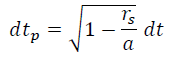
As the rates of time flow for t and tp are proportional, t=∞ is the logical equivalent of tp=∞ in all respects.
For those who doggedly insist that the probe must eventually cross the event horizon, one can always rebut, “Maybe so, but it has not happened yet". If GR is to be believed, such an event can only occur when time ceases to exist for the fixed observer. If and when that happens, the time-dependent laws of physics that we understand today will no longer apply. The fact remains that, as long as the fixed observer’s clock continues to run, the probe will remain outside the event horizon.
Full Reconciliation
Having introduced this new interpretation, what remains is to demonstrate how it perfectly reconciles with all current observations.
In related literature, we are told that once a black hole forms, it begins to accrete surrounding matter. As additional matter is drawn within the event horizon, the mass of the black hole increases, and the event horizon expands accordingly. This traditional scenario makes no sense in light of the prior analysis.
The accretion process is nothing more than that of external bodies falling into the black hole. Each piece of falling space debris behaves exactly like a falling probe. Regardless of when or where each object was released, or how fast it was moving at the time, it can never reach the event horizon. Regardless of how long we, as fixed observers, are willing to wait, we will never witness a single piece of matter crossing the event horizon.
As per equation (2) the size of a black hole is proportional to its mass. However, if nothing ever crosses the event horizon, it cannot grow. The black hole is destined to remain the same size forever. The same applies to every black hole supposedly present today. They must all be the same size they were when originally formed. This begs the question: How could the alleged black holes have formed in the first place? Consider the following thought experiment.
Dust cloud thought experiment
Assume the existence of a spherically symmetric body, such as a large dust cloud. Assume also that it is at rest with radius r=a, and that at t=0 it is allowed to collapse under its own gravitational influence. In addition, assume that there is no interaction between the particles, and thus, no internal pressure or resistance to collapse. What would we observe?
First, for reasons of symmetry, we expect that each particle will begin to fall directly toward the center. Each particle moves only along its own radial, and no angular momentum is imparted to any single particle or the body as a whole.
Second, we expect the radial motion for all particles at any given radius r<a to share the same time dependence. Particles with different radii will behave differently, but all of them at any common radius will behave the same. Therefore, we can consider the dust cloud as a set of concentric shells, each maintaining its spherical symmetry. Consequently, in this highly idealized model, we conclude that the spherical symmetry of the dust cloud is maintained for all values of t as well.
A key characteristic of the Schwarzschild metric that has not yet been discussed is its time independence. This property means that the metric remains valid even if the distribution of mass is not static, as long as spherical symmetry is maintained. It can be static, collapsing, expanding, or oscillating. The effects are identical as long as the spherical symmetry is not disturbed [11]. This means that in the current case, the Schwarzschild metric remains valid even though the dust cloud is collapsing.
The Schwarzschild metric is valid only in the region of space outside the cloud, and as such, it cannot be used to deduce the time dependence of the interior particles. However, because it is valid in the exterior region, it is correct for the particles on the outside layer of the cloud, and each particle on the surface behaves just like the falling probe previously analyzed.
Therefore, we observe that the surface falls away at an ever-increasing rate. This rate approaches, but never reaches nor exceeds the speed of light. Likewise, the total energy of the body cannot achieve an infinite value. As with the falling probe, we never experience an event where it reaches the event horizon. Because a black hole does not form until all of its matter falls within its own Schwarzschild radius, we must conclude that the black hole itself never materializes.
The evolution of black holes
If black holes are impossible, what really happens when stars die? I am not suggesting that dying stars do not collapse. They do. The formation of white dwarfs and neutron stars is well established. In addition, there is strong evidence that beyond a certain mass limit, even neutron degeneracy pressure is insufficient to maintain equilibrium. Once their fuel is exhausted, these massive objects may well experience uncontrolled collapse. What I am proposing is that even though this is likely so, true black holes never quite materialize due to a lack of time.
Heretofore, the quest to know if black holes exist has always focused on the search for physical limitations that might preclude them. Having found none, theorists have conceded that their formation must be inevitable. In contrast, I contend that black hole formation is fundamentally impossible, not because of some underlying physical effect, but because of the self-regulating nature of spacetime itself.
As a body collapses toward its own critical radius, the process slows down owing to the effect of time dilation. As the collapse proceeds, time dilation increases accordingly, further retarding the process. This tug of war continues indefinitely in such a way that ever-increasing time dilation prevents the ultimate completion of the collapsing process, regardless of the details of that process.
From a local perspective, collapse proceeds at a normal rate. From an external, fixed perspective, it is virtually frozen in time. Activities requiring only nanoseconds at the local level may well equate to billions of years from our external perspective. These two perspectives are entirely consistent with each other where the principles of GR are concerned. In neither case does the process of gravitational collapse achieve full completion.
What really happens is that the surface begins a race toward the Schwarzschild radius that it cannot win. As measured by fixed observers, the rate of collapse quickly approaches the speed of light. Because the surface is receding at nearly the speed of light, signals originating on the surface become so red-shifted that they are undetectable. At the same time, the position of the surface will approach the Schwarzschild radius so closely that fixed observers’ instruments will be unable to discern the difference. Consequently, the collapsing object will assume the effective nature of a black hole, without actually achieving that true state. Given the age of the universe, I expect that this scenario has played out literally billions of times.
Undoubtedly critics will be tempted to dismiss my ideas on the basis that we have already discovered black holes, including one at the center of our galaxy. But hang on. What is it that we really know? We know, due to the orbital motion of nearby stars, that there is an extremely massive body there, perhaps on the order of a million solar masses. We also know that this body is not detectable by existing radio telescopes because it is too small to be resolved and/or its illumination is too red-shifted to be detected. However, the conclusion that it is a genuine black hole is an inference, based on the belief that the current theory is correct. Indeed, if the current theory were correct, these observations are precisely what we would expect.
However, the model I have proposed yields precisely the same predictions. The spacetime curvature of empty space surrounding a spherically symmetric, non-rotating body that is only infinitesimally larger than its Schwarzschild radius will be the same in every way as that of an actual black hole. This is the salient point. The effects of either of these two models outside the Schwarzschild radius will be identical in every respect; not similar but identical. This includes gravitational effects on other bodies, the deflection of light, gravitational lensing, time dilation, and gravitational waves. There are simply no observational effects in the exterior region that can differentiate between the two models. My new interpretation predicts differences only with respect to the conditions on or inside the Schwarzschild radius. The validity of either model can be confirmed only by observations made within this critical radius. How or when it may be possible to collect such observational data is anyone’s guess.
Interior solution
Although the surface of a collapsing star cannot fall within its own Schwarzschild radius, it will approach that location asymptotically. This finding suggests that there is a potential dilemma. I stated earlier that the region r≤rs does not apply to GR analysis. The fact that most of a collapsing star lies inside its Schwarzschild radius raises the question of whether it is possible to analyze the conditions in that region. However, when one considers the interior solution of the Schwarzschild metric, rs no longer plays the role of a critical radius. A singular condition exists only if the Schwarzschild radius is exposed outside the actual surface of the star, a so-called naked singularity.
Most of the preceding analysis has been based on the Schwarzschild metric as defined by equation (1). It is important to understand that this metric, although it is an exact solution, is valid only in the region of free space surrounding the body of matter. The conditions inside the body are governed by an entirely different solution. Thus, investigating the conditions inside a collapsing star is not the same as investigating those inside an event horizon.
Because relativistic solutions always reduce to Newtonian results when the velocities are small and gravitational fields are weak, one can usually gain insight from Newtonian solutions. The Newtonian solution for the gravitational potential exterior to a spherically symmetric body with radius r=R is given by the following equation.
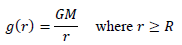
A singularity occurs at r=0, but this is a nonissue given that the equation is valid only when r≥R. The interior solution is quite different and is dependent on the mass density as a function of r. When the mass density is constant, the solution is very simple [12].
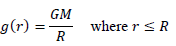
Similar to the Newtonian solution, the relativistic solution for the interior region can only be derived if one knows the mass density as a function of r. This value, in turn, depends on the relationship between density and internal pressure. Unfortunately, these relationships are not simple, and there is no generalized solution.
However, if one assumes that the density is constant, it is possible to derive an exact result. Although this result is not particularly useful in defining the actual conditions inside a real star, it does serve to illustrate those conditions at a qualitative level. The following is the metric equation for the interior region 0≤r≤R, given constant density [13].

The reader can quickly verify that this result is identical to equation (1) when evaluated at r=R. Similar to the Newtonian solution, this is a necessary condition. Examination of equation (28) in the region 0≤r≤R reveals several important points.
• None of the metric components exhibits a singularity anywhere in the region. In particular, no singularity occurs at either r = rs or at r=0. There is no true singularity at the center of the black hole as predicted by the current model.
• The manifold signature is (1,3) for all values of r. Thus, the metric characterizes a Lorentz manifold.
• The metric component of the dt2 term, g00 is always greater than zero; thus, proper time is real and nonzero for all values of r. Geodesic coordinates therefore correspond to Minkowski space throughout the region.
Combining these results with those of previous sections leads to the following generalized principle: as long as the surface of the collapsing star remains outside the Schwarzschild radius, as it must, no singular condition is encountered. Local Minkowski frames of reference can be established and the principles of GR remain valid at all physical locations both inside and outside the star. Of course, this is based on the assumption that the mass density of the star is constant, but there is no reason to expect that the qualitative result is different for any other case.
Those who are still unnerved by the idea that proper time on the falling probe approaches a finite limit as it nears the event horizon need not be concerned. In this scenario, the probe will always come into contact with the surface of the star before it reaches the Schwarzschild radius. At that point, the metric solution for the interior kicks in, and the onboard clock continues to move forward as normal. The onboard clock never stops.
Conclusion
What I have done is introduce a new model for how spacetime curvature affects the motion of material objects near the Schwarzschild radius. To be clear, the mathematical analysis is not in question. Instead, the model is based on a fresh interpretation of well-vetted mathematical results. I have shown that although the Schwarzschild metric characterizes a smooth pseudo-Riemannian manifold, only the subset of that manifold lying in the external region r > rs qualifies for GR analysis because only that region is time-orientable. Proper time is undefined elsewhere.
Existing theory predicts that a free-falling probe will pass smoothly through the event horizon. This prediction seems irrefutable, given that a smooth geodesic can be derived from any point in the manifold to the origin. However, only that portion of the geodesic lying outside the event horizon can be employed to track the motion of the probe. The arc length of the geodesic inside the event horizon does not correspond to proper time.
This leads to a far more reasonable interpretation of the probe’s behavior. Owing to the severe curvature of space and time, a probe never crosses the event horizon. This interpretation reconciles precisely with that of any fixed observer.
The Schwarzschild radius may not be a true singularity, but it is a demarcation between timelike and spacelike regions and is therefore an asymptotic choke point where the principles of GR are concerned. This is best understood as a fundamental principle. In the same way that SR precludes speeds equal to or greater than that of light, the principles of GR do not allow motion to extend beyond the boundaries of the external, time-orientable region.
Extending this logic leads to an even more important result. Instead of predicting the formation of black holes, the exact opposite is true. The same extreme curvature of space and time that prevents a free-falling probe from crossing the event horizon prevents any object from collapsing inside its own Schwarzschild radius. All the external effects of such objects are identical in every way to true, theoretical black holes. Thus, objects that appear to be black holes are those that have collapsed so closely to that state that we cannot tell the difference with external measurements.
In effect, GR predicts that there is a fundamental and absolute limit to the density of any material object. This conclusion has cosmological implications. If we run the clock backward, we may discover that the Big Bang did not originate from a singularity after all. Perhaps it originated from a timeless state of maximally compressed pure energy. Perhaps time itself began only at that moment when this maximally compressed energy began uncontrolled expansion toward the universe that we know today.
References
- Thorne KS. Black Holes and Time Warps. 1982.
- Adler R, Bazin M, Schiffer M, et al. Introduction to general relativity.
- Kenyon, I.R. General Relativity. (1990)
- Adler R, Bazin M, Schiffer M, et al. Introduction to general relativity. 222-3.
- Resnick R. Introduction to special relativity, John Willey and Sons Inc. New York. 1968:167-77.
- Resnick R. Introduction to special relativity, John Willey and Sons Inc. New York. 1968:196-9.
- Minkowski, H. The Fundamental Equations for Electromagnet Processes in Moving Bodies. (1920).
- Stover, Christopher. Semi-Riemannian Manifold. From MathWorld–A Wolfram Web Resource
- Weisstein, Eric W. Sylvester’s Inertia Law. From MathWorld–A Wolfram Web Resource
- Gardner R. Geodesics. (2016).
- Adler R, Bazin M, Schiffer M, et al. Introduction to general relativity.195.
- Symon, K.R. Mechanics, Addison-Wesley. (1964).
- Adler R, Bazin M, Schiffer M, et al. Introduction to general relativity.468-72.
- Misner CW, Thorne KS, Wheeler JA. Gravitation WH Freeman and Co. San Francisco. (1973).
Appendix A
Falling probe equations of motion
A free-falling probe follows a timelike geodesic, which can be derived using variational methods [14]. Begin with the Schwarzschild metric equation (1) and divide by dτ2 to obtain the appropriate Lagrangian function.
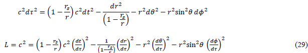
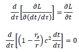
Apply the Euler-Lagrange equation with respect to θ.
Orient the coordinate system such that θ=π/2 and dθ /dτ =0 when τ=0. From this result, it is evident that these initial values are valid solutions for all τ. Therefore, motion is confined to the plane defined by θ=π/2, and the problem is reduced to two spatial dimensions. Substitute these values into equation (29).

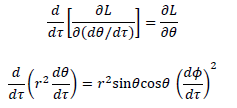
Apply the Euler-Lagrange equation with respect to t.
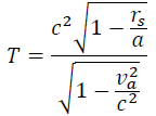
Define relativistic total energy per unit mass T as follows. Because its derivative is zero, T is a constant of motion that can be determined from initial conditions.

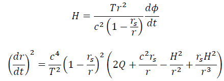
Apply the Euler-Lagrange equation with respect to φ.
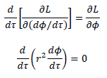
Define relativistic angular momentum per unit mass H as follows. Because its derivative is zero, H is a constant of motion that can be determined from initial conditions.
Use equations (31) and (32) to eliminate dt /dr and dφ /dτ from equation (30) and solve for dr /dτ .
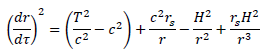
As a matter of convenience, define an equivalent constant Q as follows.
Equations (31), (32), and (34) fully describe the motion of the probe relative to proper time τ. Equation (34) is an ordinary differential equation that can, in principle, be solved for r(τ). The result can then be used in equations (31) and (32) to solve for t(τ) and φ(τ) respectively. Recall that θ=π/2 for all τ.
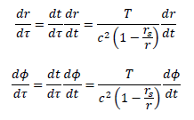
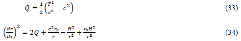
To track the motion from the perspective of a fixed observer, r and φ must be expressed as functions of coordinate time t rather than proper time τ. Use the chain rule in conjunction with equation (31) to express dr /dr and dr /dr in terms of t.
Substitute these expressions into equations (32) and (34) and simplify.
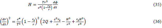
Equations (35) and (36) fully describe the probe’s motion relative to coordinate time t. Equation (36) is an ordinary differential equation that can, in principle, be solved for r(t). The result can then be used in equation (35) to solve for φ(t). Recall that θ=π/2 for all t.
Appendix B
Initial conditions
Consider a probe released at time t=0 from point P(r=a,θ=π/2,φ=0) with velocity components vr and vφ measured with respect to the local frame of reference at P. Note that vθ =0, consistent with the equations of motion derived in Appendix A. Begin by transforming to locally flat, geodesic coordinates tp, xr, xθ , and xφ , which resolve to the Lorentz metric ημν at point P.

Apply the initial conditions of reference point P(r=a,θ=π/2,φ=0) to equation (1).

Equations (37) and (38) are equivalent. Thus, the following coordinate relationships are self-evident.

Determine the local velocity components in terms of t, r, θ, and φ.
Apply the initial condition r=a to equation (35) and use equation (40) to eliminate dφ /dt .
Apply the initial condition r=a to equation (36) and rearrange.

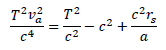
Use equations (33), (40), and (41) to eliminate Q, dr /dt , and H respectively.
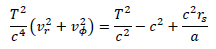
Because 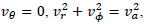 where va is the magnitude of the probe’s velocity measured locally at r=a.
Use equation (42) to eliminate T from equation (41).

Use equation (42) to eliminate T from equation (33).
Use equation (2) to eliminate rs.
Equations (42), (43), and (44) express the constants of motion in terms of the reference point and the local velocity. A few comments are in order regarding the significance of these constants and the forms in which they are expressed:
• When va≪c, equation (43) reduces to the Newtonian expression for angular momentum J/m. Thus, H is the generalized form of relativistic angular momentum per unit mass.
• When rs=2GM /c2=0 or a≫rs , equation (42) reduces to SR total energy E/m. Thus, T is the generalized form of relativistic energy per unit mass.
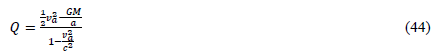
• When va≪c, equation (44) reduces to the Newtonian expression for the probe’s total energy per unit mass in a gravitational field. Thus, Q is the generalized form for relativistic energy per unit mass in a gravitational field.
• T and Q depend only on the velocity va and radial location a. This is consistent with the corresponding Newtonian values in that they do not depend on the individual velocity components or angular momentum.
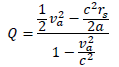
• Significant qualitative behavior of the probe can be obtained directly from equation (44). Since v<c for all material objects, the denominator is always positive. Therefore, the sign of Q is determined by the numerator. If Q<0, then the motion is bound. If H=0, then the maximum value of r occurs when v=0.
If Q>0, the motion is unbounded, and terminal velocity v occurs as r approaches infinity.
The case of Q=0 leads to a definition of escape velocity.

This expression is identical to that of the Newtonian solution. However, it must be noted that v is measured in terms of the local coordinate system at radial position r.
• Because equation (33) defines Q directly in terms of T, these two values represent alternate aspects of the same thing, namely energy per unit mass. The choice of which to use is clearly a matter of preference and should be dictated by the context. Where both terms appear in the same expression, one must remain aware of the fact that they are directly related, and thus are not independent constants of motion.
• Many authors include the mass of the probe in the definition of these constants. Expressing them as per unit mass values eliminates the probe’s mass from the equations of motion. This emphasizes that the motion of a probe in a gravitational field is completely independent of its mass.
Appendix C
Gullstrand–Painlevé coordinates
To transformation to Gullstrand–Painlevé coordinates, begin with the Schwarzschild metric equation (1).

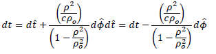
Define a new time coordinate t̂.
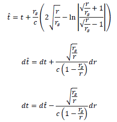
Substitute directly into equation (45) and simplify.
None of the terms in this form diverges to infinity at r = rs, thus the component singularity has been eliminated.
However, note that the transformation does not change the fact that the location r = rs is a demarcation between timelike and spacelike regions in the manifold. In particular, note what happens when the distance infinitesimals are set to zero.

Thus, as with the Schwarzschild metric, proper time is defined as a real, nonzero value only when r > rs. The region r≤rs is no more accessible to GR analysis than when using the Schwarzschild metric.
It is also instructive to observe how this transformation process applies to the rotating frame of reference illustration. Begin with equation (12).

Define a new time coordinate t.
Substitute directly into equation (46).
The reader will undoubtedly recognize this result as shown in equation (11). Thus, this transformation is simply the inverse of the derivation step between equations (11) and (12).
The parallel with Gullstrand–Painlevé coordinates is self-evident. Although the transformation eliminates the component singularity, it does not change the analysis of the rotating frame of reference. The Lorentz manifold is still divided into timelike and spacelike regions at ρ=ρ0, proper time is still defined only when ρ<ρ0, and GR analysis is still applicable only when frames of reference are moving slower than the speed of light.
Appendix D
Kruskal–Szekeres coordinates
Kruskal-Szekeres coordinates u and v are defined in terms of Schwarzschild coordinates r and t as per the following transformations. Coordinates θ and φ remain unchanged.
The salient properties of the coordinate system are shown in FIG. 4. This diagram shows how coordinates u and v relate to their counterparts r and t with θ and φ suppressed to fixed values. The region u>|v| corresponds to r > rs. The region v>|u| corresponds to r < rs. Ray u=v corresponds to the event horizon r = rs.

Figure 4: Kruskal–Szekeres coordinates.
Constant values of time t correspond to rays of constant slope radiating from the coordinate origin. The ray with slope zero corresponds to t=0. The rays of slope −1 and +1 correspond to times t=−∞ and t=∞ respectively. Thus a ray sweeping counterclockwise from slope −1 to +1 in the region r > rs corresponds to the passage of time t in a positive direction from t=−∞ to t=∞. A ray sweeping counterclockwise from slope +1 to −1 in the region r < rs corresponds to the passage of time t in a negative direction from t=∞ to t=−∞.
Constant values of r correspond to hyperbolic branches. The positive hyperbolic branches shown in blue correspond to constant values of r > rs. The positive hyperbolic branch shown in green corresponds to the value r=0 in the region r < rs.
The motivating and most significant feature of Kruskal-Szekeres coordinates is that light rays appear on the diagram as straight lines. The dashed red line with slope +1 corresponds to a light signal moving away from the origin. The dashed red line with slope −1 corresponds to a light signal moving toward the origin.