Research
, Volume: 11( 6) DOI: 10.37532/2320-6756.2023.11 (6).348On Vacuum Energy of the Universe at the Galaxy Level, the Cosmological Level and the Quantum Level
- *Correspondence:
- Engel Roza Philips Research Labs, Eindhoven, the Netherlands, E-mail: engel.roza@onsbrabantnet.nl
Received date: 24-May-2023, Manuscript No. tspa-23-99955; Editor assigned: 27-May-2023, Pre-QC No. tspa-23-99955 (PQ); Reviewed: 06June-2023, QC No. tspa-23-99955 (Q); Revised: 08-June-2023, Manuscript No. tspa-23-99955 (R); Published: 15-June-2023, DOI. 10.37532/2320-6756.2023.11 (6).348
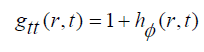
Citation: Roza E. On The Vacuum Energy of the Universe at The Galaxy Level, The Cosmological Level and The Quantum Level. J. Phys. Astron.2023;11(5):348.
Abstract
It is shown that the Lambda component in the cosmological Lambda-CDM model can be conceived as vacuum energy, consisting of gravitational particles subject to Heisenberg’s energy-time uncertainty. These particles can be modelled as elementary polarizable Diractype dipoles (“darks”) in a fluidal space at thermodynamic equilibrium, with spins that are subject to the Bekenstein-Hawking entropy. Around the baryonic kernels, uniformly distributed in the universe, the spins are polarized, thereby invoking an increase of the effective gravitational strength of the kernels. It explains the dark matter effect of galaxies to the extent that a numerical value of Milgrom’s acceleration constant can be assigned by theory. Non-polarized vacuum particles beyond the baryonic kernels compose the dark energy at the cosmological level. The result is an interpretation of gravity at the quantum level in terms of quantitatively established shares in baryonic matter, dark matter and dark energy, which correspond with the values of the Lambda-CDM model.
Keywords
Milgrom’s acceleration constant; Bekenstein-Hawking entropy; gravitational dipole; dark matter
Introduction
Present-day theory of gravity relies upon the presence of an omni-present energetic background field. The existence of this background field is required to explain the accelerated expansion of the universe, known since 1998, [1]. This cosmological background field has been defined on the basis of Einstein’s Cosmological Constant [2]. It is also known as “dark energy”. The unavoidable conclusion is that there is not such a thing as “empty space”, but that space is filled with an energetic fluidum. This conclusion has given rise to the idea of conceiving the vacuum as an entropic medium filled with energetic constituents, in this article to be annotated as darks. As long as these darks are not subject to any directional energetic influence, their motions remain fully chaotic. In that state the vacuum is fully symmetric, because it’s state before and after a time interval of “closed eyes” with an arbitrary translation or rotation of the observer, is just the same [3]. It has been argued that if the cosmological background field would consist of energetic uniformly distributed polarizable vacuum particles, the dark energy would give an explanation for the dark matter problem as well, because vacuum polarization would evoke a gravitational equivalent of the well-known Debije effect [4-9]. With the difference, though, that the central force from a gravitational nucleus is enhanced just opposite to the suppression of the Coulomb force from an electrically charged nucleus in an ionized plasma. It means that the awareness of the Cosmological Constant implies a symmetry break. This is the issue that will be discussed in this article.
The modeling of the omni-present background energy by energetic vacuum particles, requires a model for its elementary constituent (the dark). This element must be a source of energy, and must be force feeling as well. In those aspects it resembles an electron, which is ultimately the source of electromagnetic energy, and which is sensitive to the fields spread by other electrons. However, whereas the dark in the cosmological background field must be polarizable under the gravitational potential, an electron is non-polarizable under an electric potential. The electric dipole moment of an electron is zero, while a dark should have a nonzero gravitational dipole moment. Recently, the author of this article found a Dirac particle, of a particular type that, unlike the electron type, possesses a dipole moment that is polarizable in a scalar potential field [10, 11]. It is my aim to show in this article that a particle of this kind matches with the dark. The dark shares this property with the quark [12].
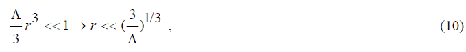
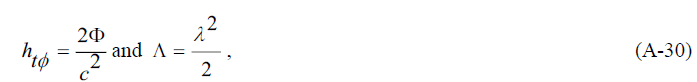
The cosmological and gravity view to be developed in this article relies, next to the awareness of the darks, on a particular interpretation of the parameter Λ in Einstein’s Field Equation. Different from the common perception that Einstein’s Λ is a constant of nature, usually identified as the Cosmological Constant, it is in the author’s view a covariant integration constant that may have different values depending on the scope of a cosmological system under consideration. This awareness is based upon Einstein’s note in his 1916 article in which he equated an integration constant as zero [13]. More on this in the next paragraph. Because it may depend on other attributes but just time-space coordinates, such as mass content, for instance, it may have different values at the level of solar systems, galaxies and the universe. Only at the latter level, it is justified to identify the Λ as the Cosmological Constant indeed. At that level, by the way, the cosmological system is in a state of maximum symmetry and maximum entropy. The viability of this view will be proven by a calculation of Milgrom’s empirical acceleration constant of dark matter [14].
In the article, first of all the need will be revealed for accepting a fluidal energetic vacuum with the profile just described. This will be done in a hierarchic approach. It is instructive to distinguish three levels in this. The first level is the galaxy level. That part contains an analysis of the dark matter problem on the basis of the role of Einstein’s Λ in his Field Equation. It will be shown that this results into a modification of Newton’s gravity law that qualitatively fits with Milgrom’s empirical one. This is possible by conceiving the galaxy as a baryonic kernel that executes a central force. The second level is the cosmological level. In this level the universe is conceived as a uniform distribution of such baryonic kernels. This will enable deriving a testable quantitative result of Milgrom’s acceleration constant. It has to be emphasized that the analysis of the two cosmological levels, i.e. galaxy and universe, does not require a microscopic identification of the vacuum energy. Accepting the role Einstein’s Λ in his Field Equation is adequate here. The third level is the other extreme: the quantum level. At that level a quantum interpretation is given for the dark energy fluid as represented by Einstein’sΛ. The purpose here is twofold. The first is to connect the Λ CDM model with entropic gravity and quantum gravity [15]. The second purpose is to strengthen the analysis made in the first and second level by showing that calculating Milgrom’s acceleration constant in a (quantum) entropic way results in an identical expression as obtained in the non- (quantum) entropic way.
In a conclusive discussion paragraph a reflection will be given on the symmetry of the universe by summarizing the analytical results from the three levels (galaxy, universe, quantum level).
The Galaxy Level
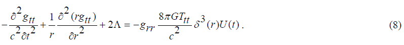
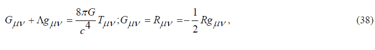
As just explained, an analysis of galaxies is the first thing to be done. To do so, Einstein’s Field Equation is invoked. The Field Equation reads as,
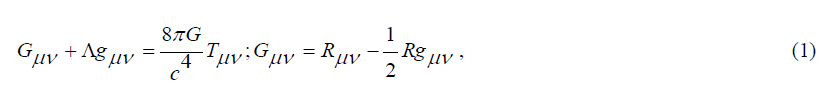
in which Tμν is the stress-energy function, which describes the energy and the momenta of the source(s) and in which Rμνand R are respectively the so-called Ricci tensor and the Ricci scalar. These can be calculated if the metric tensor components gμν are known [13, 16, 17]. The Λ term is missing in Einstein’s paper of 1916, in spite of his awareness that he equated an integration constant as zero [13]. Later, in 1917, Einstein added this quantity as a covariant integration constant for allowing vacuum solutions of his Field Equation [18, 19]. As noted in the introduction, it is usually presently taken for granted that this Lambda is a Cosmological Constant that can be regarded as a constant of nature. In fact, however, it is just a constant in the sense that its value does not depend on space-time coordinates. It may depend on attributes, like for instance mass. Hence, the Lambda may have at the galaxy level a different value from the Cosmological Constant at the level of the universe. Einstein’s Field Equation is highly nonlinear. As is well known, it can be linearized under suitable constraints and approximations, eventually even up to Newton’s law of gravity. Let us summarize the linearization and let us face the problem of a non-zero value for Λ in this.
In the case that a particle under consideration is subject to a central force only, the space-time condition shows a spherical symmetric isotropy. This allows to read the metric elements gij from a simple line element that can be written as

In which q0=ict and
t means that the number of metric elements gij reduce to a few, and that only two of them are time and radial dependent. Note: The author of this article has a preference for the “Hawking metric” (+,+,+,+) for(ict,x,y,z ) like, for instance also used by Dyson and Perkins [20,21]. By handling time as an imaginary quantity instead of a real one, the ugly minus sign in the metric (-,+,+,+) disappears owing to the obtained full symmetry between the temporal domain and the spatial one.
Before discussing the impact of Λ, it is instructive to summarize Schwarzschild’s solution of Einstein’s equation for a central point like source with mass M in empty space and 0Λ=, in which the metric components appear being subject to the simple relationship.

Solving Einstein’s equation under adoption of a massive source with point like distribution T00=Mc2 δ3(r), results in a wave equation with the format [22].
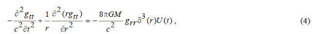
in which G is the gravitational constant and (Ut) is Heaviside’s step function.
Its stationary solution under the weak field limit,
 in which
is the well-known Newtonian potential,
The wave equation (4) reduces to,
With inclusion of the constant Λ, the wave equation is modified into (see Appendix),
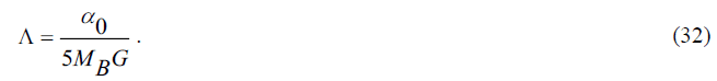
If Ttt were a point like source Ttt =Mc2 δ3(r)U(t), the static solution of this equation would be provided by the Schwarzschildde Sitter metric, also known as Kottler metric, given by [23,24],

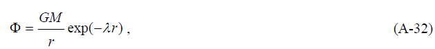
The viability of (9) readily follows by insertion into (8) and subsequent evaluation. Obviously, we meet a problem here, because we cannot separate a weak field Φ (= gravitational potential) from the metric, because we cannot a priori identify a r-domain that justifies the adoption of the constraint (5). However, given the fact that a viable wave function can be obtained for0Λ=, one might expect that it must be possible to obtain a valid wave equation for a weak field Φshowing a gradual move from 0Λ= to 0Λ. Inspection of (9) reveals that if
he Kottler metric reduces to the Schwarzschild metric. It may therefore be expected that the Einstein equation can be linearized in a spatial range between an upper limit that is set by the Kottler metric and the lower limit rRS that is set by the Schwarzschild metric. As elaborated in the Appendix, the linearization between the two limits results into a modification of the 0Λ= wave equation (7), to a 0Λ wave equation with the format
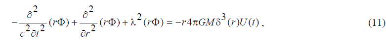
n which λ2=2Λ and in which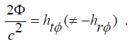
Under static conditions, (11) reduces to,
It is instructive to interpret this linearized result in terms of the non-linearized expression (8). Whereas an empty space with 0Λ= corresponds with virtual sources Tμμ=0,the vacuum with Λ ≠0 is a fluidal space with virtual sources

with gμμ=(1,1,r2 sin2 ϑ,r2)[25-27].Owing to the Hawking metric, is equal for all diagonal elements). This particular stressenergy tensor with equal diagonal elements corresponds with the one for a perfect fluid in thermodynamic equilibrium [28]. Inserting a massive source in this fluid will curve the vacuum to gμμ=(gtt,grr,r2 sin2 ϑ,r2).Hence, inclusion of theΛ implies that, under absence of massive sources, Einstein’s equation can be satisfied if empty space is given up and is replaced by a space that behaves as a molecular fluidum in thermodynamic equilibrium. If, under bias of a uniformly distributed background energy, a massive pointlike source is inserted into this fluidum, deriving a meaningful wave equation is possible. The perception that in this thermodynamic equilibrium space-time is still uncurved and that curving is the result of a disturbance on it makes the ormat of the wave equation shown by (11) different from the formats reviewed in [29,30]. It corresponds with what is presently known as “emergent gravity”, in which the disturbance of the entropy on the thermodynamic equilibrium is seen as the origin of gravity [31,32].
As noted before, and well known of course, Poisson’s equation and its modification is the static state of a wave equation. From the perspective of classic field theory, a wave equation, can be conceived as the result of an equation of motion derived under application of the action principle from a Lagrangian density Lof a scalar field with the generic format

in which U(Φ) is the potential energy of the field and where ρΦ is the source term. Comparing various fields of energy, we have,
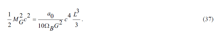
U(Φ)=0 for electromagnetism
U(Φ)=-λ2 Φ2/2 for electromagnetism
U(Φ)=λ2 Φ2/2 for the nuclear force [33].
The non-trivial solutions of wave functions) in homogeneous format derived from (14), for the first case and the third case, are respectively,
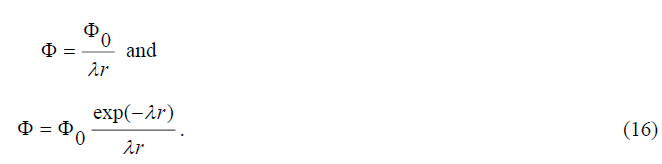
The first case applies to electromagnetism ( for Φ0=Qλ/4 πε0) and to Newtonian gravity( for Φ0=MGλ). The third case applies to Proca’s generalization of the Maxwellian field [34]. The latter one reduces to the first case if λ →0,while keeping Φ0/λ constant. Generically, it represents a field with a format that corresponds with the potential as in the case of a shielded electric field (Debije [9]), as well as with Yukawa’s proposal, to explain the short range of the nuclear force [33].
Let us, after this side-step, proceed on (12). It can be readily verified that this equation can be satisfied by,
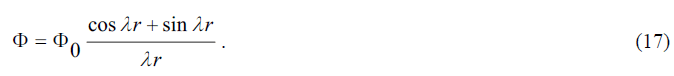
Note that the goniometric shape of this solution is a consequence of the plus sign in front of λ2. It has to emphasized once more that this expression holds under the classical weak field constraint and the presence of a central source of energy that evokes this field as the tiny variation in the generic spherical metric. The shape (17) will reveal some interesting features. In accordance with the concepts of classical field theory, the field strength can be established as the spatial derivative of the potential Φ . We may identify this field strength as a cosmological gravitational accelerationg. Let us compare this acceleration with the Newtonian one gN.
Hence, from (17),

Not surprisingly, the gravitational acceleration is affected by the Einstein’s Λ=λ2/2. If Λ=0, the gravitational acceleration equals the Newtonian one gN. Under a positive value of Lambda, the gravitational acceleration has a different spatial behavior. This is illustrated in FIG. 1 which shows the ratio g / gN as a function of the normalized spatial quantity λr. Up to the value λr=3π/4,g / gNrises monotonously up to the value g / gN=3.33. This figure shows that, for relative small values ofr, the cosmological acceleration behaves similarly as the Newtonian one. Its relative strength over the Newtonian one increases significantly for large values of r , although it drops below the Newtonian one at λr > 3.45. Up to slightly belowλr=3π/4 , this is, as will be shown, a similar behavior as heuristically implemented in MOND. The effective range is determined by the parameter λ. Let us consider its consequence.
Newtonian laws prescribe that the transverse velocity vφ(r) of a cosmic object revolving in a circular orbit with radius r in a gravity field is determined by

Figure 1: The cosmological gravity force compared with the Newtonian force.
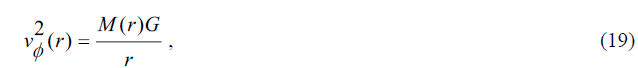
in which M(r) is the amount of enclosed mass. This relationship is often denoted as Kepler’s third law. Curiously, like first announced by Vera Rubin [35] in 1975, the velocity curve of cosmic objects in a galaxy, such as, for instance, the Milky Way, appears being almost flat. It is tempting to believe that this can be due to a particular spectral distribution of the spectral density to compose M(r) . This, however, cannot be true, because M(r)builds up to a constant value of the overall mass. And Kepler’s law states in fact that a flat mass curve M(r) is not compatible with a flat velocity curve. FIG. 2 illustrates the problem. It is one of the two: either the gravitational acceleration at cosmological distances is larger than the Newtonian one, or dark matter, affecting the mass distribution is responsible. Cosmological gravity as expressed by (18) may give the clue. Its effective range is determined by the parameter λ. It might therefore well be that the cosmological gravity force manifests itself only at cosmological scale. FIG. 3 shows that under influence of this force, the rotation curves in the galaxy are subject to a boost. This cosmological gravity shows another intriguing phenomenon. Like shown in FIG. 1 and FIG. 4, at the very far cosmological distance, the attraction of gravity is inversed into repulsion [36-38]. This repulsion shows up at the very far end of the spatial range. It prevents the clustering of the fluidal space, thereby eliminating the major argument against the fluidal space approach.

Figure 2: Incompatibility of a flat enclosed mass curve with a flat rotation curve. Note: for illustration purpose a particular distribution is adopted for the enclosed mass. The same distribution is maintained for all subsequent illustrations.

Figure 3: Boost of the rotation curve under influence of cosmological gravity.

Figure 4: Inversion of the gravity force to antigravity at large cosmological distances. Black: Newtonian. Blue: Cosmological Gravity.
Further exploration of this phenomenon is a subject outside the scope of this article. It has to be noted that the solution (19) is not unique. There are more solutions possible by modifying the magnitude of sin λr ver cos λr . I have simply chosen here for the symmetrical solution. Cosmological observations would be required to obtain more insight in this.
Whether this theoretically derived modification of the Newtonian gravity indeed explains the excessive orbital speeds of stars in a galaxy, such as formulated in Milgrom’s empirical law in MOND, is dependent on the numerical value of Einstein’s Λ . If Milgrom’s empirical theory and the one developed in this paragraph are both true, it must be possible to relate Einstein’s Λ with Milgrom’s acceleration constant α0 , like will be done next.
Comparison with MOND
MOND is a heuristic approach based on a modification of the gravitational acceleration g such that
 , with
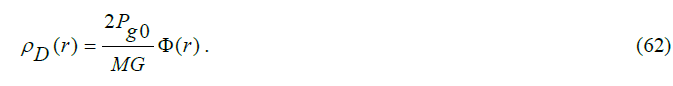
in which μ(x) is an interpolation function, gN(=MG/r2) the Newtonian gravitational acceleration and in which a0 is an empirical constant acceleration. The format of the interpolation function is not known, but the objectives of MOND are met by a simple function like [14,39].
If g/a0<<1, such as happens for large r , (20) reduces to

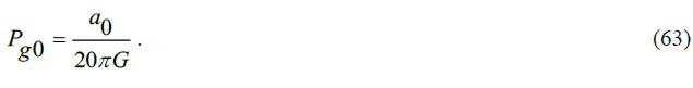
Under this condition, the gravitational acceleration decreases as r-1 instead of r-2. As a result, the orbital velocity curves as a function of r show up as flat curves.
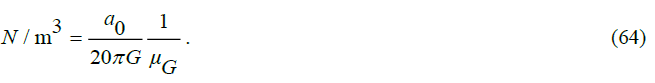
Algebraic evaluation of (20) and (21) results into,
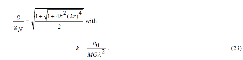
This expression allows a comparison with (18).
As illustrated in FIG. 5. a pretty good fit is obtained between (18) and (23) in the range up to λr=3π/4 (where the theoretical curve starts decaying), if

Figure 5: MOND’s interpolation function compared with the theory as developed.

Observations on various galaxies have shown that a0 can be regarded as a galaxy-independent constant with a value about a0≈1.25×10⁻¹⁰m/s2[40].
The implication of (24) is, that a0 is a second gravitational constant next to G . The two constants determine the range λ of the gravitational force in solar systems and galaxy systems as λ2≈2 a0/5MG, in which M is the enclosed mass in those systems. Whereas this second gravitational quantity a0 is an invariable constant, this is apparently not true for the Einsteinian parameter Λ.
This result shows that Milgom’s empirical law and the theory as developed in this article are intimately related. FIG. 6 shows the difference between the curves for the orbital velocity of stars in galaxies according to MOND as compared to those as predicted by the theory as developed in this article. It has to be emphasized here that establishing the fit between the two curves by setting k=2.5 is only meant to incorporate Milgrom’s acceleration constant as an unknown parameter into the theory. This implies that no limitation on whatsoever is imposed, nor that the generality of the analysis is affected. From FIG. 5 it is shown that beyond rλ =3π/4 the developed theory deviates from MOND and FIG. 4 shows that beyond rλ=3.66 the gravitational attraction changes into a repulsion. From this perspective, the latter phenomenon would even put a natural limit to the size of a galaxy.

Figure 6: Comparison of orbital velocities for stars in galaxies for MOND (upper curve) and for the theory as developed (lower curve).
Let us consider these ranges for the Milky Way. As long as λr<3π/4 we have

This implies a spatial coincidence range between MOND and the theory developed so far, up to a galaxy radius RM to the amount of
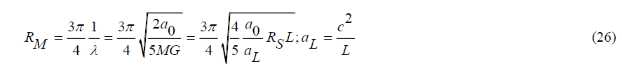
where RS=MG/c2 is the Schwarzschild radius and L=ctH is the Hubble scale (tH=13.8Gyear) aL≈6.9×10⁻¹⁰m/s2 and because aL≈1.25×10⁻¹⁰m/s2 from MOND’s assessment to most galaxies (if not all), we have from (26) for the Milky Way with Schwarzschild radius RS≈0.2 lightyear,
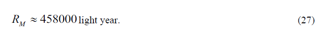
This is well beyond the radius of the Milky Way, which amounts to 180.000 - 200.000 lightyear. The coincidence range between MOND and this theory (up to rλ=3π/4) is well within the spatial validity range , due to the weak field limit constraint and the linearization approximation such as derived in the Appendix.
As noted before, apart from this upper limit for the range of validity, there is a lower limit as well. This has to do with the weak field limit constraint that we have imposed to derive a single parameter wave equation from Einstein’s Field Equation. The value of this lower limit has been derived in the Appendix as
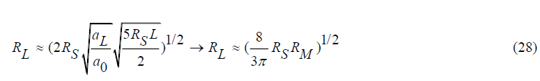
For the Milky Way (RS≈0.2 lightyear; RM≈458000 lightyear) this lower limit amounts to
RL≈279 lightyear. (29)
Considering that our solar system is at about 26.000 lightyear from the center, it will be clear that the modified Newtonian gravitation law (18) holds for the Milky Way. Because many other galaxies are similar to the Milky Way, it is quite probable that this new theory solves the anomaly problem of the stellar rotation problem of most, if not all, galaxies.
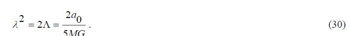
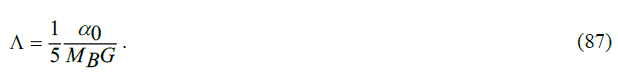
From this result it may be concluded that that Milgrom’s acceleration constant and Einstein’s Λ are closely related indeed. From (25) and (11), we have
It also means that Einstein’s Λ is not a constant of nature, but instead, like noted before, a covariant integration constant that, while being independent of space-time coordinates, may be dependent on attributes of any cosmological system that is subject to Einstein’s Field Equation. If the system is a spherical one, such as solar systems or galaxies, the value of Einstein’s Λ depends on the baryonic mass content of the system under consideration.
The Cosmological Level
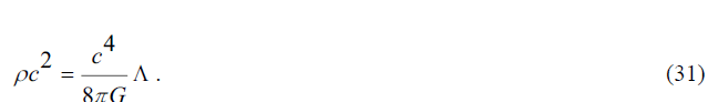
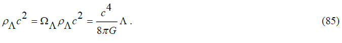
So far, we have considered a spherical gravitational system under influence of a central gravitational force, such as applies to solar systems and galaxies. But what about the universe? For any observer in the cosmos, the universe is a sphere with distributed matter. Let us model the universe as a sphere in the cosmos with radius L and distributed gravitational energy. We have discussed before that the vacuum is fluidal space with virtual sources Tμμ=-ρΛ,in which ρ=c4/8πG. Denoting the gravitational background energy density as ρ , we have
We have concluded before that Λ is related with some baryonic mass MB,such that
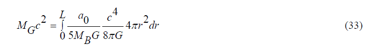
The distributed energy is a gradually developed mixture of the energy from fluidal matter as meant by (31) and the energy from baryonic matter MB as meant by (32). From these expressions it can be concluded that the total gravitation energy MGc2 in a sphere with radius Lcan be expressed as
Let ΔMGthe difference between the gravitational matter in a sphere L+ΔL and the gravitational matter in a sphere L.It follows readily that
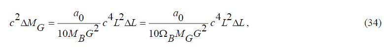
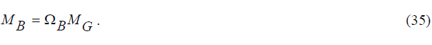
in which the baryonic matter is expressed as a dimensionless fraction ΩB of the gravitational matter,
Note: In terms of the Lambda-CDM nomenclature, the baryonic share is expressed as ΩBin the relationship

In which Ωm,ΩΛ,ΩB,ΩD, respectively, are the relative matter density, the relative dark energy matter density, the relative baryonic matter density and the relative dark matter density [17]. While the matter distribution between the matter density Ωm(=0.259) and dark energy density ΩΛ(= 0.741) is largely understood as a consequence from the Friedmann equations that evolve from Einstein’s Field Equation under the Friedmann-Lemairtre-Robertson-Walker (FLRW) metric, the distribution between the baryonic matter density ΩB(= 0.0486) and dark matter density ΩD(= 0.210) is empirically established from observation [17,40]. The quoted values are those as established by the Planck Collaboration [15].
Eq. (34) can now be integrated as
Hence, the gravitational energy density ρc2in the sphere with radius L is given by
Because the visible universe is a sphere from which light cannot escape, its radius equals the Schwarzschild radius [41],
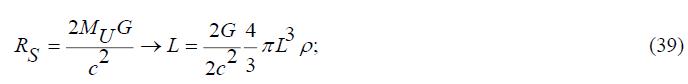
in which MU is the total gravitational mass of the universe and in whichis the overall matter density of the universe. Hence, from (38) and (39),
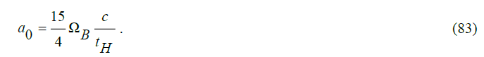
Identifying L like before as the Hubble scale L=ctH(tH=13.8 Gyear),we aL≈6.9 ×10⁻¹⁰m/s2 and inserting the empirical Λ CDM value ΩB=0.0486 the into this expression gives the well-known value a0≈1.25×10⁻¹⁰ m/s2 for Milgrom’s acceleration constant. It is a result that relates the baryonic content of the universe with Milgrom’s constant by a rather simple expression. It makes the theory developed so far testable by experimental observation, such as required for its viability.
The Three Components of the Gravitational Matter
The baryonic energy density is just one of the three components of the gravitational energy. What about the other two components? These are known as common knowledge that can be found in textbooks [42]. For properly relating the dark matter content found in the previous paragraph, it is instructive to give a short summary.
To do so, let us inspect Einstein’s Field Equation (1) once more,

and let the metric of the spherically modelled visible universe be the well-known FLRW metric [17], defined by the line element,

in which q0=ct is the normalized time coordinate , and where k is a measure for the curving of space-time. The scale factor ()atexpresses the time-dependence of the size of the universe. The ratio
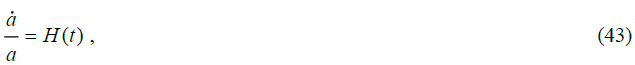
is known as the Hubble factor. It is the main observable of the universe, because its numerical value can be established from red shift observations on cosmological objects (a=da/dt).
The solutions of (43) under constraint of the metric (42) are [40],
The awareness that the vacuum is not an empty space, but, instead a fluidal space with virtual sources Tμμ=-Λc2/k, where k=8πG/c2[25,26,27]- owing to the Hawking metric, Tμμis equal for all diagonal elements - , will modify the two Friedmann equations [40] that originally have been conceived for empty space. This can be summarized as follows. First, the term Λgμvis moved to the right side of (41), such that it can be conceived as additional contributions to the energy density p(t)and the fluid pressure p(t),
Under the constraint k=0 (flat universe), and taking into consideration (44a,b), the first Friedmann equation evolves as,
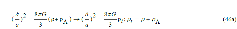
The second Friedmann equation reads as,

Differentiating the mass density ρt in (46a) gives,
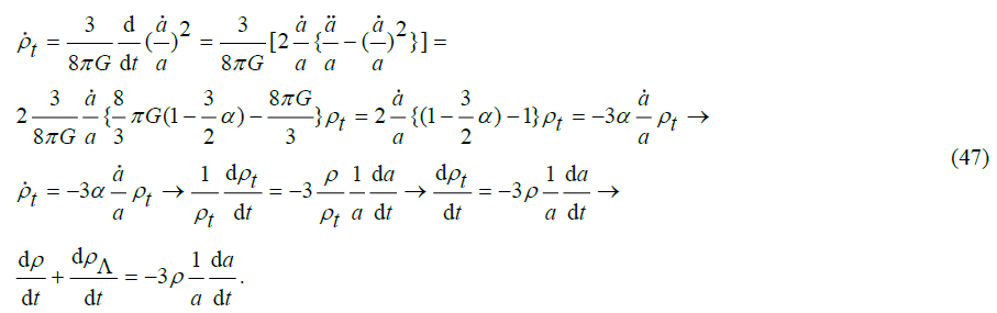
Because the background massive density ρΛ is time-independent (Λ is independent of space-time coordinates), (47) is satisfied if,
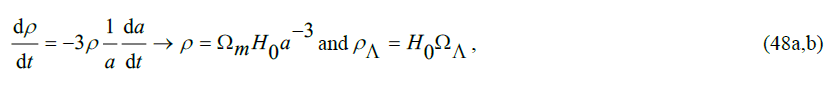
in which Ωm,ΩΛand H0are constants. The quantity H0 is the Hubble parameter a/a at a(t)=1. It is tempting to believe that Ωm and ΩΛare, respectively, the relative amount of baryonic mass ρ/ρt and the relative amount of background mass ρΛ/ρt at a(t)=1. This, however, is not necessarily be true, because (without further constraints) the differential equation (48) is satisfied for any distribution between Ωm and ΩΛ as long as Ωm+ΩΛ=1.
Applying (48) on the first Friedmann equation (45a), results into,
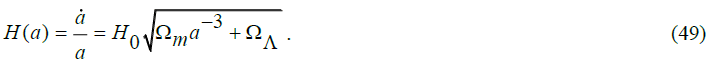
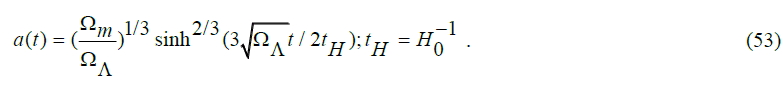
This equation represents the Lambda-CDM model in its most simple format (actually, more terms are heuristically added under the square root operator to model empirical evidence from certain cosmological phenomena). Eq. (49) can be analytically solved as [43, 44].
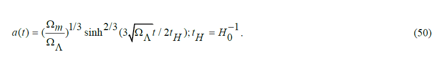
At present time t=tp the scale factor equals unity (a=1) and the Hubble parameter is the observable H0.Equating present time tpwith Hubble time tHis justified if a(t) would have shown a linear increase over time up to now, under a constant rate of say c0.because in that case a(t)=c0t and a(t)=c0.This is Hubble’s empirical law. Equating tp=tH in (50) as an axiomatic assumption, indeed results in a behavior of the scale curve that, up to present time t≤tH, is pretty close to Hubble’s empirical law. Hence, from (49),
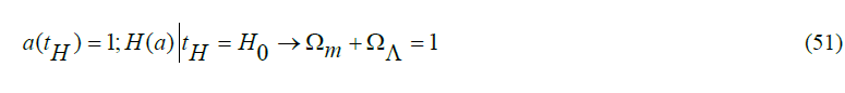
Hence, from (50) and (49),
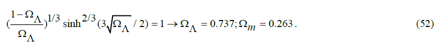
These values are only slightly different from those in the six-parameter Lambda-CDM model (where Ωm=0.259).The difference is due to the simplicity of the format (49), in which only matter and dark energy is included. For more precision, the radiation contribution from the cosmic microwave background (CMB) should be taken into account as well.
FIG. 7. Demonstrates the viability of the axiomatic assumption to equate present time with Hubble time.

Figure 7: The scaling factor a(t) as a function of cosmological time. The lower curve represents Hubble’s law. The upper curve shows the curve of accelerated scaling due to Einstein’s Cosmological Constant.
Summarizing:
The time behaviour of the scaling factor of the universe is a solution of Einstein’s Field Equation under the FRLW-metric,
As a consequence of a(tH)=1, the relative values for matter density and dark energy are established as,

The relationship between Milgrom’s acceleration parameter and the ratio BΩ of baryonic matter over gravitational matter has been established before as,
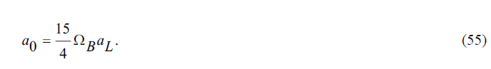
Accepting the life time of the universe tH=13.8 Gyear and a0=1.256 ×10⁻¹⁰m/s2 as primary independent quantities, we get ΩB=0.0486. This makes the dark matter content ΩD=Ωm-ΩB-0.263-0.0486=0.214
The Quantum Level
In spite of now having obtained by theory testable numerical values for dark matter and dark energy, the true physical nature of these components has remained unclear. All we know so far is, that the universe is apparently filled with an energetic fluid that has got a mathematical abstraction in Einstein’s Field Equation in terms of virtual sources Tμμ=-ρΛ, with ρ=c4/8πG.The issue to be addressed next is the question whether it is possible to give a physical profile to these constituents of the energetic background fluid. Let us conceive these constituents as vacuum particles in a state of Heisenberg unrest. Let us denote these particles as darks and let us suppose that these darks show a polarizable dipole moment in a scalar potential field. Like already discussed before, a background fluid with polarizable dipoles executes a shielding effect on a scalar potential. It may suppress its strength, like in the case of the potential field of a electrically charged particle in an ionic atomic plasma (Debije effect) or enhance its strength, like in the case of modified gravity as explained in before in this article (section 2). Let us try to obtain a density expression for these vacuum particles (darks). To do so, let us rewrite (12) as,

and subsequently into,
∇2Φ=-4πGρ(r), in which
In Debije’s theory of electric dipoles [6,9,45],

The vector Pg is the dipole density. From (58),
Assuming that in the static condition the space fluid is eventually fully polarized by the field of the pointlike source,Pg(r) is a constant Pg0, Hence, from (59),
Taking into account that to first order,
we have from (60) and (61),
Hence, from (30), (57) and (60-62),
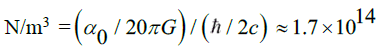
By assigning an elementary dipole moment μG to the dark, the volume density N/m3 of the darks is found as,
Profiling the Dark
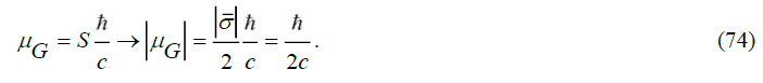
Let us suppose, just by hypothesis, that the origin of this elementary dipole moment is a result of an elementary quantum mechanical vibration in a similar way as the elementary angular momentum ħ of a Dirac particle can be visualized as an elementary virtual rotation. This vibration would create a spatial Heisenberg uncertainty d around its supposed position, which can be explained as the result of a motion with ultra-relativistic speed near vacuum light velocity c in an Heisenberg time interval Δt such that
d=cΔt. (65)
Applying Heisenberg’s relationship ΔEΔt=ħ/2, [46], on (65), we get

in which μG has the dimensions of a (mass) dipole moment expressed in terms of Planck’s reduced constant and the vacuum light velocity c. The virtual mass mshould not be confused with the particle’s rest mass0m. To some readers this may seem a bold an unjustified hypothesis. However, quite recently it has been proven that Dirac’s theory of electrons allows a rigid formal theoretical basis for the hypothetical existence of elementary particles with a (second) quantum mechanical dipole moment ħ/c next to the angular (first) quantum mechanical dipole moment ħ. More precisely, Dirac’s theory predicts, next to the electron-type a noncanonical type with the unique property of showing a real dipole moment with magnitude,
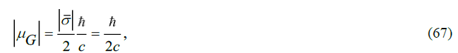
in which σ is the Pauli vector, and which, unlike the two other ones, is polarisable in a scalar potential field [10,11]. Originating from the Heisenberg uncertainty, this polarisable dipole moment is a pure quantum mechanical phenomenon. Its dipole mass is unrelated with the rest mass of the particle. The rest mass may have any value, down to an extremely tiny quantity, while leaving the dipole moment unaffected. This property fits well to the gravitational “dark” as just described. The results from [11] applied to a dark can be summarized as follows.
Like all elementary fermions, a dark has to follow Fermi-Dirac statistics, should obey the Pauli Exclusion Principle and should have half integer spin. They can be modelled with the Dirac equation. The canonic formulation of Dirac’s particle equation reads as [47-49],
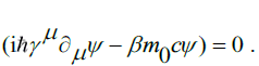
In which m0 is the particles rest mass, β a 4 x 4 unity matrix and in which the 4 x 4 gamma matrices have the properties,

While the canonical set of gamma matrices is given by,

he γ-set of the non-canonical type is defined as,

In which σ i are the Pauli matrices. Moreover this non-canonical set is subject to the more severe constraint [13],

Note that this set is obtained from the canonical Dirac set by making the γ0 set imaginary and by replacing the β matrix into the “fifth gamma matrix”. The set is an improvement of the erroneous one reported in [10, eq. (27)], for which the author is indebted to prof. D. Zeppenfeld. For this reason [10] has got an update as [11].
Although the wave equation of the electron type and that of the non-canonical type are hardly different, there is a major difference in an important property. Both have two dipole moments. A first one, to be indicated in this text as the angular dipole moment, is associated with the elementary angular momentum ħ. The second one, to be indicated as the polarisable dipole moment is associated with the vector ħ/c. These dipole moments show up in the calculation of the excess energy of the particle in motion subject to a vector potential A(A0,AX,AY,AZ) . In the canonical case (69a) we have,
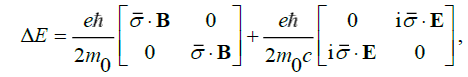
in which σ is the Pauli vector, defined by

in which (i,j,k) are the spatial unit vectors and in which B and E are generic field vectors derived from the vector potential. The redundancy in (70) allows writing it as,
The electron has a real first dipole moment (eħ/2m0), known as the magnetic dipole moment, and an imaginary second dipole moment (ieħ/2m0c), known as the anomalous electric dipole moment. The spin vector  has an eigen value
  . In the case that the Dirac particle is of the non-canonical type as defined by (69b), we have [11],

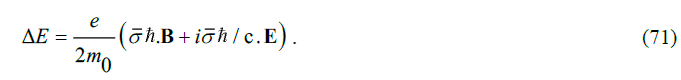
The non-canonical type Dirac particle has two real dipole moments, generically, i.e., without identifying it as an electromagnetic ones, to the amounts of σħ respectively σħ/c . If the dark would be of the electron type, it would not be polarisable in a scalar potential field, because such a field is Coulomb-like and is unable to polarize an imaginary electric dipole moment. If, however, the dark is a non-canonical type, its second dipole moment can be polarized under influence of a scalar potential field. This field is not necessarily the electromagnetic one. The coupling factor eis not necessarily the elementary electric charge. If the field is just a scalar potential, eq. (72) can be written as,
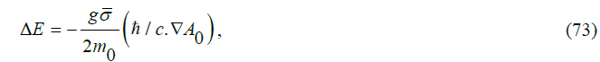
in which g is a generic coupling factor, which in the case of a gravitational particle just equal to mo. Hence, taking into account that the eigen value is of the spin vector is related with the state variable
 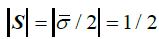 , the polarisable dipole moment μG of a dark in a scalar nuclear field ∇A0 is given by,
Summarizing: conceiving the dark as a non-canonical type Dirac particle allows considering the dark as a particle that, under influence of its dipole moment, can be polarized in a (scalar) gravitational potential field. FIG. 8. illustrates the difference with the electron.

Figure 8: Like all Dirac particles, the dark has two anomalous dipole moments, a first one due to an elementary angular momentum and a second one due to an elementary linear momentum h/ c . While in the case of an electron the latter one is a dynamic one with a zero static value, it is a static one in the case of a dark.
Note that, whereas other authors [4, 6], describe gravitational dipoles as structures with positive and negative mass ingredients, the dipole described here is a virtual vibrating particle. To some readers it may seem that I am introducing here a new kind of matter. This is not true. The vibrating particle is part of the vacuum energy, modelled as an ideal fluid in thermodynamic equilibrium that emerges from Einstein’s Lambda in the solution of his Field Equation of the vacuum [27, 49]. The equilibrium state of the fluid itself is irrelevant. Hence the gravitational molecules show up as a vibration of the vacuum. This is different from novel matter of baryonic nature.
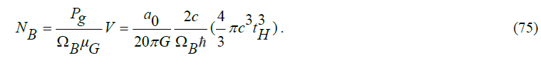
Taking (64) and (74) into account, the amount of baryonic darks in a spatial volume V equal to the size of the universe amounts to,
Gravitational Entropy
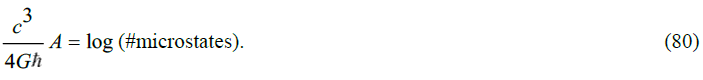
Because the dipole moments of the darks can only assume two quantized values (bits), this number (75) represents the total information content of the universe. Like shown by Verlinde [32, 50], the information content can be established as well from quite a different viewpoint. The Bekenstein-Hawking expression for the entropy of a black hole is a first ingredient for calculation. It reads as [32, 50],
in which cis the vacuum light velocity, Gthe gravitational constant, Planck’s (reduced) constant, Athe black hole’s peripheral area and kB is Boltzmann’s constant. The peripheral area of a spherical black hole is determined by its Schwarzschild radius as,
in which M is the baryonic mass of the black hole. Boltzmann’s constant shows up as a consequence of the thermodynamic definition of entropy. In that definition SH is not dimensionless, because of the thermodynamic interpretation of entropy as a measure for the unrest of molecules due to temperature, which relates the increase ΔS of entropy with an increase molecular energy ΔE due to temperature T, such as expressed by the thermodynamic definition,
ΔE=TΔS. (78)
Boltzmann’s famous conjecture connects entropy with information, by stating
SB=kBlog(#microstates). (79)
This conjecture expresses the expectation that entropy can be expressed in terms of the total number of states that can be assumed by an assembly of molecules. Boltzmann’s constant shows up to correct for dimensionality. I would like to emphasize here that (76) and (79) are different definitions for the entropyS, and not necessarily identical. Knowing that (76) has been derived from (78) and accepting Boltzmann’s conjecture, we would have,
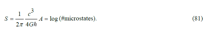
Both sides of this expression are dimensionless. Omitting Boltzmann’s constant makes entropy a dimensionless measure of information, which, of course, is very appealing. At this point, I wish to elaborate on a subtlety, which has been shown by Verlinde. According to Boltzmann’s conjecture, an elementary step ΔS in entropy would imply ΔS =kB Verlinde has proven, however, that an elementary step in entropy from the Hawking-Bekenstein entropy implies ΔS =2πkB. If not, the Hawking-Bekenstein’s formula would violate Newton’s gravity law [50]. Because Boltzmann’s expression is a conjecture without proof, the problem can be settled by modifying the dimensionless expression of entropy (73) into,
Considering the well-known relationship between the event horizon ctH of the visible universe and the Schwarzschild radius from the critical mass enclosed within that horizon (tH is the Hubble time scale) that allows conceiving the visible universe as a virtual black hole [41]. The entropy within the event horizon of the universe can be established as
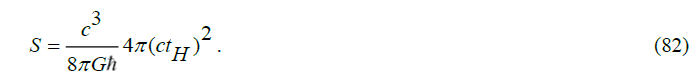
Equating (82) with (75) gives,
This is just the same expression as (55), which has been derived from quite a different point of view. This identity proves the viability of both approaches, thereby strengthening the validity of the theory developed in this article.
Summarizing: the energetic background fluid in the universe is built up by quantum particles. These quantum particles have a polarisable dipole moment μG with an eigen value to the amount of μG . The volume density of these quantum particles as calculated from (64) amounts to N/m3 = 1.7 x 1041 or, equivalently, 1.7 x 10¹⁴ particles per cubic nanometer. This makes the energetic background fluid rather smooth. From this volume density and the critical matter density of the universe the mass of these particles can be calculated.
The critical mass density ρc can be expressed in terms of Hubble time tH from the consideration that the universe is a bubble from which light cannot escape. Hence as a black hole with radius RS=ctH, such that

It gives 9.4 10-27 kg/m3. Divided over 1.7 x 1041 particles, it gives a mass of 5.55 10-68 kg per particle, which corresponds to a massive energy of 3 10-32 eV. This makes the darks virtually mass less.
Discussion
While under adoption of Hubble’s law and the FLRW-metric the relationship between matter (DΩ) and dark energy (ΛΩ), as expressed by (52-55) is a straightforward consequence of Einstein’s Field Equation, such as established in the Lambda-CDM (ΛCDM) model of the Planck collaboration group [38], the relationship between dark matter (DΩ) and baryonic matter (BΩ) is in ΛCDM empirically assessed. In this article, I have given it a theoretical basis. A crucial element in this, is the interpretation of Einstein’s Λ in his Field Equation. Usually, this quantity is considered as a constant of nature. In the context of ΛCDM its value is established from (44) as a relationship between Λ and gravitational matter, such that
From (84) and (85),

This expression assesses a numerical value of Einstein’s at the level of the universe. At this level it makes sense to indicate this value as the Cosmological Constant. Although this quantity is a measure for the gravitational energy in the universe its magnitude is very small. This small value shows about a difference of about 120 orders of magnitude with the zero-point energy suggested by quantum field energy [51]. This discrepancy is known as “the Cosmological Constant catastrophe. In the view as discussed in this article, the magnitude of the Cosmological Constant is a result from the linearization of Einstein’s Equation with a removal of the background bias. It has to be taken into account, however, that in quantum field theory such a removal is required as well. This removal is known as renormalization.
In this article, though, I have demonstrated in this article that in the application of Einstein’s Field Equation at the level of solar systems and galaxies Einstein’s , while being a constant indeed in terms of independence of space-time coordinates, depends on the baryonic matter contentMBof the system under consideration, such that
The dependence on the baryonic matter content is obviously present at the level of the universe as well, although it remained hidden as part of the critical mass content in the considerations (85-86). It wouldn’t be correct to analyse the universe, as a simple spherical system with a central gravitational force, as if it were a huge galaxy. The universe is a distributed assembly of such spherical subsystems. It is for that reason that the critical mass of the universe, has been related in (33) to distributed baryonic kernels as fractions of gravitational matter. This not only allows assigning a numerical value to the constant0, but it also allows establishing it as a true cosmological invariant as a second gravitational constant next to the Newtonian G Curiously, whereas Einstein’s is not a true cosmological constant, Milgrom’s acceleration seems to be. It has to be noted, though, that the description of the universe in the few simple parameters 0 ,G and tHis a status quo in the sense that there is no guarantee that the numerical values of the first two of these are true invariants over cosmological time, nor that Hubble’s law has been true back to the big bang.
Conclusion
The visible universe is a space filled with energetic vacuum particles that inherit their energy from their Heisenberg uncertainty in spatial position. It are virtually mass less (≈3 10-32 eV) gravitational quantum particles that possess a polarisable dipole moment with an eigen value /2c In free state, the particle density is particles per cubic nanometer, in which 0is a true cosmological invariant, with a numerical value equal to Milgrom’s empirical acceleration constant for dark matter. If all these dipole moments were randomly orientated, the universe would show a perfect symmetry. The major part of these dipole moments (≈74%) s randomly oriented indeed, because these don’t feel a polarisable influence from a baryonic cluster. This part composes the dark energy of the universe. A significant part still (≈21%)of the polarisable dipole moments are polarized around baryonic clusters. This part, with its frozen symmetries, composes the dark matter, which enhances the gravitational strength of the baryonic clusters. The baryonic clusters are densely packed energetic particles that composes the observable baryonic matter(ΩB ≈5%) of the universe. This amount is related with Milgrom’s constant as ΩB=4tHα0/15c.
It might well be that the anti-dogmatic views on Einstein’s Lambda and on the constituting elements of the energetic background energy may meet opposition. However, as shown in this article, these starting points allow a consistent derivation by theory of two important results, which so far are only established as empirical quantities. The first is a simple formula for Milgrom’s acceleration constant, derived by theory from the two starting points. It says that a0 =(15/4)ΩB(c/tH). In most articles on Milgrom’s constant, the analysis is restricted to spherical systems with a centric force. Those articles are subject to criticism because of that reason. In this article, I have demonstrated that the analysis can be extended to a universe with distributed matter. The second important result is the calculation by theory of the matter distribution in the universe in terms ΩB+ΩD+ΩΛ=1(resulting into 0.0486 + 0.210 + 0.741 = 1). The two results taken together can be viewed as a testable solution for the dark matter problem.
Appendix: Constraints On the Linearization of Einstein’s Field Equation
The main reason of including the appendix is to show the validity range for the weak field limited modification of Newton’s gravitation law, due to Einstein’s gauge constant. To do so properly, the derivation requires a short summary of common textbook stuff without, before extending it to meet the objective. This objective implies that we have to solve Einstein’s Field Equation for a spherically symmetric space-time metric that is given by the line element (2),

in which q0=ict.
Note: The space-time (ict, r,ϑ,φ) is described on the basis of the “Hawking” metric (+,+,+,+)Once more, I would like to emphasize its merit that, by handling time as an imaginary quantity instead of a real one, the ugly minus sign in the metric (-,+,+,+) disappears owing to the obtained full symmetry between the temporal domain and the spatial one.
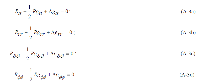
The components Gμμ compose the metric tensor gμv, which determine the Ricci tensorRμv and the Ricci scalar R. These quantities play a decisive role in Einstein’s Field Equation, which reads as

In a space without massive sources, the Einstein Field Equation under this symmetric spherical isotropy, reduces to a simple set of equations for the elements Rμμ of the Ricci tensor,
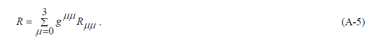
Let us proceed by considering the Ricci scalar. It is defined generically as

In spherical symmetry the matrices contain diagonal elements only, so that (A-4) reduces to
his result can be applied to (A-3). Multiplying the first one with g00(=gtt), the second one with g11, etc., and subsequent addition results of the terms μ=1,2,3 gives,
Repeating this recipe for gμμ(=1/gμμ), we have for reasons of symmetry
(this result can be checked in ref. [52], under “equivalent formulations”).
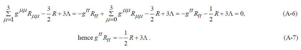
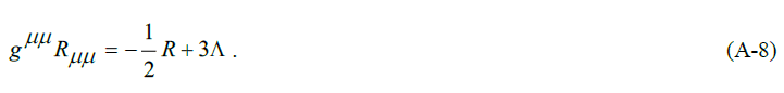
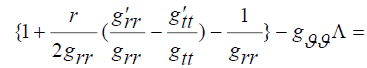
Note that the subscripts and superscripts 00, 11, 22, and 33 are, respectively, identical to tt, rr,ϑϑ and φφ. Applying this result to Einstein’s equation set (A-2), gives
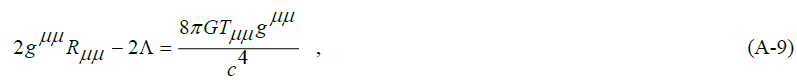
Such that after multiplication by gμμ, we have

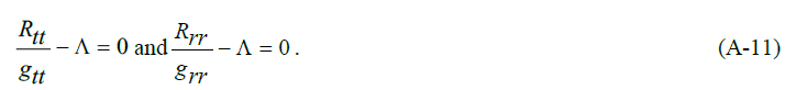
As long as Tμμ is a pointlike centric source, like assumed in the remainder of this text, this expression is consistent with the relationship Rμμ-Λgμv=0 for empty space.
Let us first proceed under the conditions of the absence of massive sources (Tμμ=0) and let us consider the Ricci tensor components Rtt and let us consider the Ricci tensor components Rrr under use of the results shown in TABLE A-1, that can be found in basic textbooks [53]. Note: g and g means differentiation, respectively double differentiation of g intor; gand g means differentiation, respectively double differentiation of g in to t. Multiplying (A-3a) by 1/gtt and (A-3b) by 1/grr gives
TABLE A-1. Metric tensor and Ricci tensor.
| Metric tensor | Ricci tensor |
|---|---|
| gtt=g00 |  |
| grr=g11 | 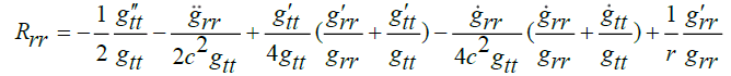 |
| gϑϑ=g22=r2 | 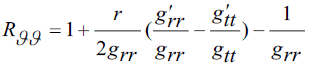 |
| gφφ=g=33=r2sin2 ϑ,r2 | 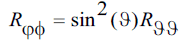 |
which, under the assumption of a zero Cosmological Constant (Λ=0), after subtraction and under use of the expressions in TABLE A-1 results into.
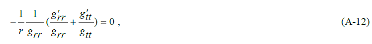
Hence
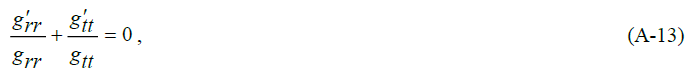
which can be integrated to (the Schwarzschild condition),

This, in turn, gives
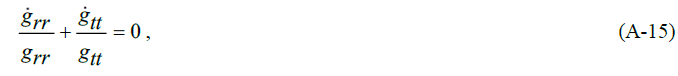
Using (A-13), (A-15) and the Table A-1 values on Rttgives

Hence, from (A-10) and (A-16) ,
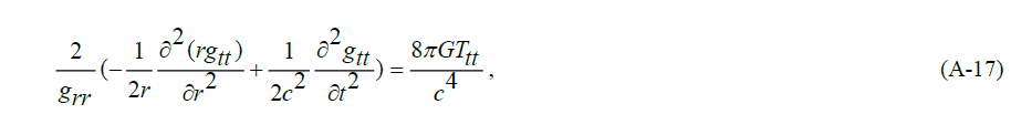
or, equivalently,
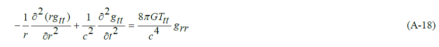
Applying well-known conditions,
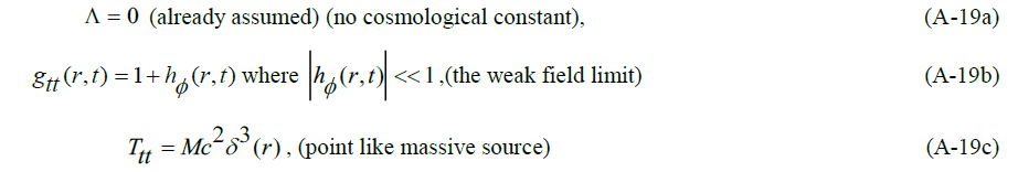
yields the proper wave equation,
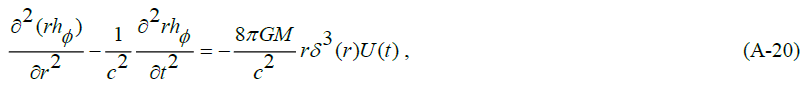
where U(t) is Heaviside’s step function. In the static regime, the equation results into
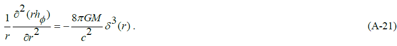
This is similar to Poisson’s equation,
the solution of which is the Newtonian potential,
Comparing (A-20) with (A-22) gives the equivalence
So far, this is just textbook stuff, such as can be found, for example, in [16]. It is needed as a basis for deriving the conditions under which the modification of the Λ=0 wave equation (A-20) toward the Λ=0one shown in (11) is justified. Let us first consider the case Λunder absence of a massive source. Obviously, (A-10) is only satisfied if the influence of the cosmological constant is counter balanced by the hypothetical source.
Because all four members of the Einstein set (A-10) have to be satisfied, we have, under consideration of (A-10) and Table A-1,
This particular stress-energy tensor with equal diagonal elements corresponds with the one for a perfect fluid in thermodynamic equilibrium. So, whereas empty space corresponds with virtual sources Tμμ=0 the fluidal space corresponds with virtual sources Tμμ=-ρΛ with gμμ=(1,1, r2 sin2 ϑ,r2) . Insertion of a massive point like source in this fluid and modifying (A-17) by adding the virtual sources, after redefining the weak limit condition as,
gives, for the static parts,
and, secondly,
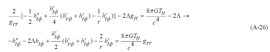
Note: Omitting the addition of the virtual sources shown in the right-hand part of the upper line of (A-26) would give the Kottler-de Sitter metric as the solution of Einstein’s equation for a point like source in empty space. Inserting the virtual sources will give an equation for a point like source in a space filled with a energetic fluid that, without the source, is in a thermodynamic equilibrium that does not curve space-time. It is the same consideration as invoked in cosmology for modifying the Friedmann equations due to Einstein’s Lambda, expressed by eq. (45) of the main text (see also [26,27]). Within the scope of this article it is the instrument that allows the linearization of Einstein’s Field Equation within a spatial range bounded by a lower limit and an upper limit.
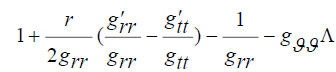
As long as Λ=0 and assuming a point like source embodied in Ttt, the Schwarzschild condition shows up. This is obvious by subtracting the latter equation from the former one, thereby allowing exclusion of a singularity at r=0. It reveals that, under this condition, the homogeneous formats of the two equations are identical. However, because this is no longer true for Λ≠0, we have to cope with two equations. These two equations are non-linear. However, because htφ and hrφ are small in the weak field limit, the two equations can be linearized under the condition that the last term in the left-hand part of these equations is dominant over their preceding terms. This assumption, to be checked later, allows to rewrite (A-26) for r≠0, as

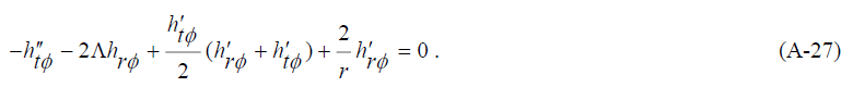
A simple format for the second equation is obtained after subtraction (A-27) from (A-26), resulting into,

Obviously,hrφcan be calculated as soon as htφ is found as a solution of (A-28). Re-inserting the pointlike source, similarly as in the case Λ=0 and including the time derivatives, yield a wave equation as a generalization of (A-28). After rewriting,
we have from (A-28) the inhomogeneous generalization,

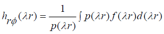
If Λ< 0 , we have under static conditions, a similarity with Helmholtz’ equation with the screened Poisson’s equation, the solution of which is Yukawa’s potential,
which reduces to Poisson’s one for λ→0.
If Λ>0 , we have under static conditions, a similarity with Helmholtz’ equation with a characteristic solution,

This solution reduces to Poisson’s one for λ→0 as well.
This is the weak field limit solution of Einstein’s Equation if one does not take the validity of Poisson’s equation of gravity for granted, but adopts Helmholtz equation instead for Λ>0.
We are not done yet. There are two remaining issues. The first one is the justification of the linearization approximation by moving from (A-26) to (A-28). Moreover, we have to take into consideration that, although the derived gravitational potential field satisfies (A-3a) and (A-3b), we are not sure that it satisfies (A-3c) and (A-3d) as well. It should do, to prevent violation of the metric (A-1). Assessment of it is the second thing to be done.
The remaining issues: (a) the linearization approximation
The linearity approximation (A-26)→(A-28) is justified as long as
Under consideration of (A-29), it can be written as,
This condition enforces calculation of hrφ from htφ. From (A-29),
This first order differential equation for hrφ can be readily solved, albeit that the resulting analytical expression from the generic solution
 in which

is a rather complicated one.
FIG. 9. illustrates the behavior of the calculated -hrφ as a function of λr compared with htφ. From (A-36), it is obvious that if λr→0,hrφ≈-htφ.The vertical axis is normalized to a dimensionless quantity, by writing, under consideration of (A-30) and (A-33),

Figure 9:Relative values of the metric quantities htφ (black) and -hrφ (blue) as a function of . λr The red curve represents the function in the right-hand part of (A-36).

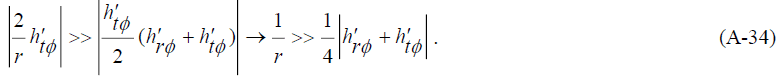
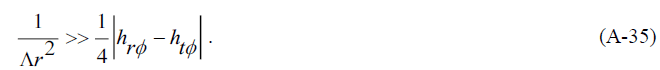
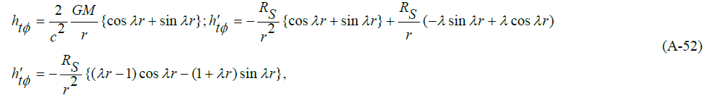
Note that RS is the Schwarzschild radius of the cosmological system (with central force) under consideration. The black curve shows the normalized value of htφ. It is gradually decreasing by r-1.The blue curve shows the normalized value of hrφ as calculated from the differential equation (A-36). This quantity tend to explode with increasing λr Nevertheless, the functions on both sides of (A-36) remain the same and show the gradual finite behavior, shown by the red curve. The reason is due to sign differences between the left-hand part and the right-hand part of (A-35). Subtraction of two large quantities makes the result still small enough. Nevertheless, the exponential increase of λr may violate the linearization approximation. This requires proper investigation. Because eventually (for relatively large λr ) hrφ>>htφ, and considering that 2Λ=λ2 , we may reformulate (A-35) as,
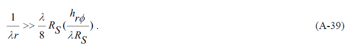
Hence, the cross over value λr0 is determined as,
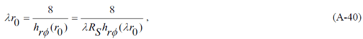
where hrφ(λr) s given by (A-37). From (A-39) it is obvious that as long as hrφ<<1 the upper limit is far beyond λr=8 However, because of the exponential growth of hrφ/λRs with λr the limit can be shifted near to this limit or even shifted below. This may spoil the weak field limit assumption. Hence, the actual validity range of the linearization heavily depends on the value of the product λRs. Once this product is known, the cross-over value of λr0 and the associated value of the metric component hrφ can be calculated from the known curve hrφ/λRs shown in FIG. 9. Because of its exponential growth, the upper limit for λr that justifies the linearization approximation, is below, but probably near, to the cross-over value.
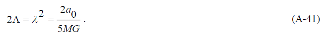
The assessment of a meaningful quantitative value to the product λRs is possible by invoking the value of Einstein’s Λ or cosmological systems with a central mass. As shown in the main text, this is obtained by the application of the theory to Milgrom’s MOND, expressed by eq. (30). This expression relates Einstein’s Λ with Milgrom’s acceleration constant a0 as,
Hence,
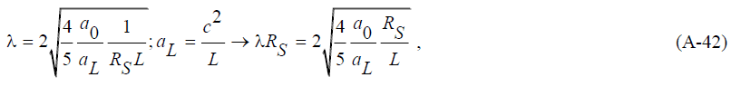
in which aLis the gravitational acceleration constant at distance Lfrom the centre of the cosmological system under consideration. Choosing Las the Hubble range L=ctH and defining c2/L=aL as the acceleration at the verge of the Hubble range, and considering that Milgrom’s acceleration constant amounts a0≈1.25 ×10⁻¹⁰m/s2 aL/a0 amounts to,aL/a0≈6.9/1.25 = 5.52. The Schwarzschild radius RSof a typical galaxy, like the Milky Way, is about 0.2 lightyear, while the Hubble time amounts to tH≈13.5 Gyear.Hence, typically

From (A-42), (A-40) and (A-37), it is found that the cross-over λr0 amounts to

The associated value of the metric component amounts to hrφ=1.01 . That violates the weak field approximation. However, at λr=6 the metric component is drops to hrφ=0.017. Hence, It is fair to say that, up to a normalized spatial distance near to λr0≈6, the derived gravitational wave equation (A-31) for galaxies akin to the Milky Way maintains its validity.
The remaining issues: (b) the other two equations
Before appearance of the massive source, we have for (A-3c),
 background matter,
in which 
After appearance of the massive source, we have
 background matter plus source,
in which
Due to the change of curving by the source, we have,

Under the constraint of the weak field limit, this equation can be rewritten as,

As long as Λgϑϑ is close to Λr2, the metric (A-1) maintains it validity. This is true as long as

The split into two conditions is made for ease of analysis. Under consideration of (A-29), (A-49b) can be rewritten as,

Because with increasing λr the quantity hrφis dominating over htφ,(A-50) can be replaced by

Thereby concluding that the condition (A-49b) is covered by the weak field constraint.
Now we have established an upper spatial limit that justifies the linearization condition and concluded that the (isotropy) condition (A-49b) is covered by the weak field constraint, we are left with a single issue. That is condition (A-49a). Considering that,
we have for (A-49a),
Hence,
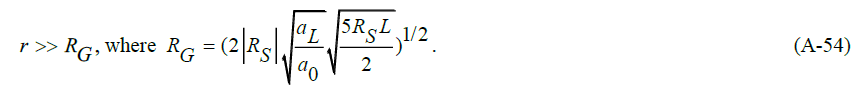
As already noted, the Schwarzschild radius RSof a typical galaxy, like the Milky Way, is about 0.2 lightyear. For such a galaxy, the range RGcalculated from (A-54) appears beingRG 278 lightyear. Considering that the radius of the Milky Way is estimated as 100.000-180.000 lightyear and that our solar system is at about 26.000 lightyear from the center, it will be clear that the wave equation (A-31) holds for the major part of the galaxy, thereby solving the anomaly problem of the stellar rotation problem.
REFERENCES
- Frieman JA, Turner MS, Huterer D. Dark energy and the accelerating universe. Annu Rev Astron Astrophys. 2008 ;46:385-432.
- Peebles PJ, Ratra B. The cosmological constant and dark energy. Reviews of modern physics. 2003;75(2):559.
- Dark energy and the accelerating universe
- Blanchet L. Dipolar particles in general relativity. Classical and Quantum Gravity. 2007;24(14):3541.
- Blanchet L, Le Tiec A. Dipolar dark matter and dark energy. Physical Review D. 2009;80(2):023524..
- Hajdukovic DS. Is dark matter an illusion created by the gravitational polarization of the quantum vacuum?. Astrophysics and Space Science. 2011;334(2):215-8.
- Penner AR. Gravitational anti-screening as an alternative to the Λ CDM ΛCDM model. Astrophysics and Space Science. 2016; 361:1-5.
- Roza E. The vacuum polarization paradox and its solution. Astrophysics and Space Science. 2019;364(4):73.
- Debye P, Huckel E. De la theorie des electrolytes. I. abaissement du point de congelation et phenomenes associes. Physikalische Zeitschrift. 1923;24(9):185-206.
- Roza E. On the second dipole moment of Dirac’s particle. Foundations of Physics. 2020;50(8):828-49.
- Roza E. On the second dipole moment of Dirac’s particle. 2020;50(8):828-49. .
- Roza E. From Black-Body Radiation to Gravity: Why Neutrinos are Left-Handed and Why the Vacuum is not Empty.2023; 11(5):341
- Einstein A. Relativity: The Special and General Theory. H. Holt and company, NY.1920.
- Milgrom M. A modification of the Newtonian dynamics as a possible alternative to the hidden mass hypothesis. Astrophysical Journal.1983;270:365-70.
- Collaboration P. Cosmological parameters. Astronomy and Astrophys. 2015;594: A13.
- Weinberg S. Gravitation and cosmology. John Wiley & Sons Inc. New York. 1972.
- d'Inverno RA. Introducing Einstein's relativity. Introducing Einstein's relativity by RA D'Inverno. New York: Oxford University Press. 1992.
- Einstein A. Sitzungsber. Cosmological Considerations on the General Theory of Relativity. Preuss Akad Wiss Berlin (Math. Phys.). 1915; 831:1915.
- Einstein A. Prinzipielles zur allgemeinen Relativitätstheorie. Annalen der Physik. 1918;360(4):241-4.
- Dyson FJ, Derbes D. Advanced quantum mechanics. World Scientific; 2011.
- Perkins DH. Introduction to high energy physics. CAMBRIDGE university press; 2000.
- Moore TA. A general relativity workbook. Mill Valley: University Science Books; 2013.
- Kottler F. Uber die physikalischen grundlagen der Einsteinschen gravitationstheorie. Annalen der Physik. 1918;361(14):401-62.
- Sun LF, Yan ML, Deng Y, et al. Schwarzschild–De Sitter Metric and Inertial Beltrami Coordinates. Modern Physics Letters A. 2013;28(29):1350114.
- Schutz B. A first course in general relativity. Cambridge university press; 2022.
- Carroll SM, Press WH, Turner EL. The cosmological constant. Annual review of astronomy and astrophysics. 1992;30(1):499-542.
- Sola J. Cosmological constant and vacuum energy: old and new ideas. In Journal of Physics: Conference Series 2013; 453(1): 012015.
- Hawking SW, Ellis GF. The large scale structure of space-time. Cambridge university press; 2023.
- Norton JD. The cosmological woes of Newtonian gravitation theory.1999.
- Harvey A, Schucking E. Einstein’s mistake and the cosmological constant. American Journal of Physics. 2000;68(8):723-7.
- Jacobson T. Thermodynamics of spacetime: The Einstein equation of state. Physical Review Letters. 1995;75(7):1260.
- Verlinde EP. Emergent gravity and the dark universe. SciPost Physics. 2017;2(3):016.
- Yukawa H. On the interaction of elementary particles. I. Proceedings of the Physico-Mathematical Society of Japan. 3rd Series. 1935; 17:48-57.
- Proca AL. Sur la theorie ondulatoire des electrons positifs et negatifs. Journal de Physique et le Radium. 1936;7(8):347-53.
- Rubin VC, Ford Jr WK, Thonnard N. Rotational properties of 21 SC galaxies with a large range of luminosities and radii, from NGC 4605/R= 4kpc/to UGC 2885/R= 122 kpc. Astrophysical Journal.1980; 238:471-87.
- Minkevich AV. On Gravitational Repulsion Effect at Extreme Conditions in Gauge Theories of Gravity. Acta Physica Polonica B. 2007;38(1).
- Luongo O, Quevedo H. Self-accelerated universe induced by repulsive effects as an alternative to dark energy and modified gravities. Foundations of Physics. 2018; 48:17-26.
- Etkin V. Gravitational repulsive forces and evolution of universe. Journal of Applied Physics. 2016;8(6):43-9.
- Gentile G, Famaey B, de Blok WJ. THINGS about MoND. Astronomy & Astrophysics. 2011;527: A76.
- Friedmann A. Uber die krümmung des raumes. Z Phys. 1922;10:377-86.
- Pathria RK. The universe as a black hole. Nature. 1972;240(5379):298-9.
- Liddle A. An introduction to modern cosmology. John Wiley & Sons; 2015.
- Wolfram S, Mathematica AW. Redwood City.1991.
- Google Scholar
- Gonano CA, Zich RE, Mussetta M. Definition for polarization P and magnetization M fully consistent with Maxwell's equations. Progress in Electromagnetics Research B. 2015; 64:83-101.
- Tamm IE, Mandelstam L, Tamm I. The uncertainty relation between energy and time in non-relativistic quantum mechanics. Selected papers. 1991:115-23.
- Dirac PA. The quantum theory of the electron. Proceedings of the Royal Society of London. Series A, Containing Papers of a Mathematical and Physical Character. 1928;117(778):610-24.
- Bjorken JD, Drell SD. Relativistic quantum mechanics. Mcgraw-Hill College. 1964.
- Carroll SM. The cosmological constant. Living reviews in relativity. 2001;4(1):1-56.
- Verlinde E. On the Origin of Gravity and the Laws of Newton. Journal of High Energy Physics. 2011;2011(4):1-27.
- Adler RJ, Casey B, Jacob OC. Vacuum catastrophe: An elementary exposition of the cosmological constant problem. American Journal of Physics. 1995;63(7):620-6.
- Cross Ref
- Carroll D. Spacetime and Geometry: An Introduction to General Relativity .Addison Wesley. San Francisco. 2004.
- The cosmological constant and dark energy