Research
, Volume: 11( 7) DOI: 10.37532/2320-6756.2023.11(7).363Method for in-field user calibration of MEMS accelerometer using hybrid genetic algorithm
- *Correspondence:
- Sok Hun Kim Faculty of Mathematics, Kim Il Sung University, Pyongyang, Democratic People's Republic of Korea, E-mail: KUC727@star-co.net.kp
Received date: 14-July-2023, Manuscript No. tspa-23-106198; Editor assigned: 17-July-2023, Pre-QC No. tspa-23-106198 (PQ); Reviewed: 24July-2023, QC No. tspa-23-106198 (Q); Revised: 26-July-2023, Manuscript No. tspa-23-106198 (R); Published: 30-July-2023, DOI. 10.37532/2320-6756.2023.11(7).363
Citation: Kim S H, Jong S B, Jong G J, et al. Method for In-Field User Calibration of MEMS Accelerometer using Hybrid Genetic Algorithm. J. Phys. Astron.2023;11(7):363.
Abstract
The Inertial Measurement Unit (IMU) using MEMS sensor contains 3-axis accelerometer, 3-axis gyroscope, 3-axis magnetometer, thermometer, etc. in a single microchip, but the installing axes are not ideally perpendicular to each other and calibration is needed. This paper describes the approach to the static calibration of an accelerometer without using any mechanical equipment on the basis of the fact that the norm of MEMS accelerometer outputs measured in the static position is ideally equal to 1. By using genetic algorithm, we verified the initial values of scale factors and zero bias ones. Taking these as the initial values of the Sequence Quadratic Programming (SQP), we found the optimal solution. We proved the effectiveness of the calibration using the measurements of MEMS accelerometer in the static position. The experimental result shows that the static calibration approach using the estimated Hybrid Genetic Algorithm (HGA) is better than the others.
Keywords
MEMS accelerometer; Auto-calibration; Genetic algorithm; SQP; BiasIntroduction
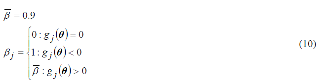
Navigation is the law to determine the position, velocity and attitude of a moving body in the space and in practice navigation parameters such as position, velocity and attitude are determined using accelerometer and gyroscope.
With the rapid development of MEMS technology, light and low-cost inertial sensors that have low power consumption are made and widely used in different sectors in our life [1-3].
Since the Inertial Measurement Unit (IMU) using MEMS sensor contains 3-axis accelerometer, 3-axis gyroscope, 3-axis magnetometer, thermometer, etc. in a single microchip, we can realize a good navigation.
However, these 3-axis sensors are not ideally perpendicular to each other, so we have to calibrate them before use [4, 5].
Calibration can be defined as a process of comparing sensor outputs with known reference information and determining coefficients that make the output agree with the reference information over a range of output values.
Calibration in use is classified into mechanical equipment based calibration, semi-mechanical calibration and calibration without external equipment.
Mechanical equipment based calibration needs an expensive turntable so many approaches to calibrate at any place without using mechanical equipment are widely studied in the world [6-10].
In general, in order to calibrate an accelerometer IMU is located in different random positions and the parameters of misalignment, zero bias and factors are computed so that the measurements of acceleration may be equal to the known reference value.
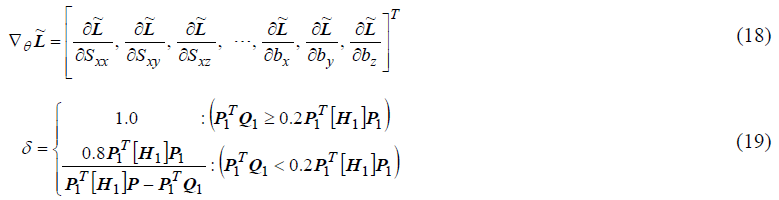
The main idea of calibration of an accelerometer is that the norm of 3-axis accelerometer outputs is equal to the acceleration of gravity, g in the static positions [3].
Using this idea, we can only measure the output of MEMS accelerometer at random directions. On the basis of the measurements of the accelerometer measured at every moment in the static positions and gravitational acceleration the error model is made. And then the parameters of the model, that is, scale factors, zero biases and non-orthogonal errors are determined so that the values of errors may get less.
I. Frosio and I. Skog proposed a calibration method in which the first search was done with Newton’s method on the basis of the assumption that there’s no cross-coupling influence between the sensor axes. The result of this search was regarded as the initial values in the case of the cross-coupling to perform the second search [2, 3].
In order to guarantee the convergence of a solution, scale factors and zero biases of a sensor were found at 30 random directions. The experiment showed the mean error of the calibrated accelerometer was always less than 2˚ and the maximum standard deviation was less than 3˚. Newton’s method, however, needs the operation of the second derivative, has a narrow convergent zone and is sensitive to the initial values.
In order to overcome these disadvantages they proposed a calibration approach by Levenberg-Marquardt (LM) nonlinear optimization which is the combination of Gradient Descent Method and Gaussian-Newton’s method.
When this calibration approach was used in the experiment, the mean square error was less than 1.5×10⁻⁴ g.
This approach also has its own disadvantages. The variance of the mean square error gets bigger according to the initial values. With the development of artificial intelligence technology, the genetic algorithm is used in optimization, control and the calibration of sensors [4].
The genetic algorithm uses the principle of the genetic evolution that a population with high adaptability, in the course of evolution, survives, but the population with low one becomes extinct.
We applied iteration method less than 25 times to get 9 parameters of non-orthogonal errors, scale factors and zero biases using genetic optimization method, and proved through simulation that the mean value of errors is less than 3.5×10⁻⁵ g. and the standard variance is less than 1.6×10⁻⁵ .
This method improves the correctness of path computation 250 times higher than the case without any calibration, and guarantees the computation correctness 10 times compared with the algorithm with 6 parameters.
Theoretically the genetic algorithm is a probable search method and it has already been proved that the optimal solution can be found with the probability of 1, but in the real application early convergence occurs so that the same individual is searched iteratively.
Consequently the path error becomes bigger exponentially after over 20 seconds. The combination of optimization methods such as genetic algorithm, Newton’s method and Quasi-Newton’s method makes it possible to overcome this drawback.
In the paper we proposed an approach to optimal solution by using the hybrid genetic algorithm that is the combination of genetic algorithm and Sequence Quadratic Programming (SQP).
We proved the effectiveness of the calibration by applying the measurements of MPU 9250 MEMS accelerometer that we found in the static positions. The result of the experiment shows that the mean square errors of the sensor model parameters are smaller than the other calibration approaches. When the test is done on the ground vehicles with the calibrated accelerometer, the navigation errors were much less than the case with uncalibrated accelerometer. The experimental result shows that when the accelerometer is calibrated using the hybrid genetic algorithm, the computation accuracy of orientation is higher than the other calibration approaches. When the calibrated accelerometer is used, the estimation accuracy of orientation can be increased in Attitude and Heading Reference System (AHRS) [11].
Calibration Principle of MEMS Accelerometer
The simple structure of an IMU is shown in FIG. 1.

Figure 1: Simplified Scheme of an IMU.
As shown in FIG. 1, if all the sensors are installed perpendicularly to each other, then each sensor measures only the acceleration in the direction of the axis on which the sensor is installed.
But for the real inertial measurement unit it is difficult for each sensor to form an ideally orthogonal frame, which is shown in FIG. 2.

Figure 2: Relation between the accelerometer orthogonal frame
In FIG. 2,α ij is the rotation of the ith sensor axis of the accelerometer about the jth axis of a platform.
Therefore, the transformation matrix from the Accelerometer Orthogonal Frame (AOF) to the Accelerometer Body Frame (ABF) is as follows.
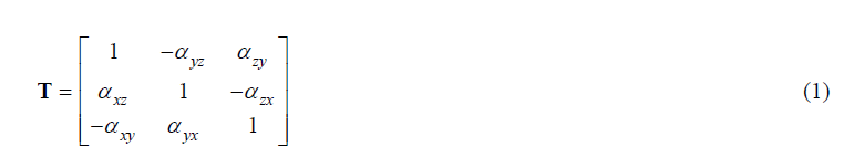
Considering Eq. (1), the measurement model of an accelerometer can be written as follows [4].

Where ao the acceleration is vector in (AOF)and aM is the acceleration vector in (ABF).
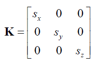 is the matrix of scale factors.
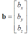 is the vector of biases.
nis assumedas themeasurement noise vector which is zero mean white Gaussian noises.
Measurements are averagedin time to removerandom errors:

In Eq. (3) o a isthe average accelerationvectorinAOF and M a is the average measured acceleration vector in ABF The main idea of calibration of an accelerometer is that the norm of 3-axis accelerometer outputs is equal to the acceleration of gravity, g in the static positions [3].
When the accelerometer is in a stationary position, the vector o a is equal to the gravitational acceleration vectorg, andwecan rewrite Eq. (3) as follows.

Modern digital MEMS accelerometers data are not read in ms-2, but in the units ofg.
Consequently, the norm of the vector of gravitational acceleration vector becomes 1 and the Eq. (4) can be written as follows.

The measurements averaged in quite different positions of the accelerometer are taken.
Using Eq. (5) and the data from these measurements, the fitness function can be defined as follows:

Where 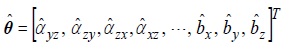 are the parameters to be evaluated,aiM is the vector of average measurements in different positions and N is the number of positions.
In-field Calibration of MEMS Accelerometer using Hybrid Genetic Algorithm
Design of hybrid genetic algorithm
Genetic algorithm, as one of the optimal search methods, which is the imitation of biological evolution, has got a discontinuous objective function or singular point, and it can be used to solve various optimization problems.
In practical application, however, genetic algorithm has got some drawbacks.
One of the drawbacks is that due to the early convergence, the same individual is iteratively searched. Therefore, even though the optimal solution range is found, the capability of local search within the range is very weak. On the contrary, some optimization methods such as gradient method and Newton’s method have got very strong capability of local search.
Therefore, if you configure hybrid genetic algorithm using this optimization method in search of genetic algorithm, you can improve the execution efficiency and the quality of the genetic algorithm. In the paper we are going to determine the calibration parameters to calibrate MEMS sensors using the hybrid genetic algorithm that is the combination of genetic algorithm and sequence quadratic programming. FIG. 3 shows the block diagram of the designed hybrid genetic algorithm.

Figure 3: Block diagram of hybrid genetic algorithm.
When you add the local search to the genetic algorithm, you can improve the overall performance of the population by making a local search on the basis of the phenotype corresponding to each individual of the population and by finding the local optimal solution in the existing situation of each individual. Also, you can perform the operation of the next-generation genetic evolution on the basis of a new population by coding the local optimal solution obtained in the course of local search and transforming them into new individuals.
Execution process of the hybrid genetic algorithm;
Step 1: Initialization of the number tof evolution generation, that is, t=0
Step 2: Production of initial population P(t) randomly
Step 3: Fitness evaluation of the population P(t)
Step 4: Selection of individual and crossing-over by crossover probability Pc: P(t) ← Crossover [ P(t) ]
Step 5: Mutation by probabilitym Pm: P"(t) Mutation [ P'(t) ]
Step 6: Execution of SQP: P"t ←SQP [ P"(t) ]
Step 7: Fitness evaluation of the population P"(t)
Step 8: Selection of individual and reproduction:P(t + 1)←Reproduction [P(t)∪P"(t) ]
Evaluation of stopping condition: if the stopping condition is not satisfied, take t←t+1 and go back to step 4.
If the stopping condition is satisfied, output all the optimal individuals finalize computation.
Each stage of the genetic algorithm is set as follows.
Size of population: 300, Encoding: floating number encoding
Fitness function: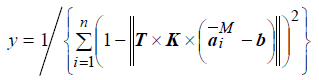
Scale transformation: Sequence transformation
Selective operation: Tournament selection, Crossover operation: Algebraic crossover, Mutation: Real number mutation operator Stopping criterion: in case that the change in the best fitness functions is less than 10-15when the maximum generation number reaches 200 or within 70 generations.
Search for local optimal solution using sequence quadratic programming
Step 1: Setting of the problem of quadratic programming with linear limit to determine the search direction and its solution
From the data of sensor we can see the upper and lower limits to establish the following restrictive conditions.
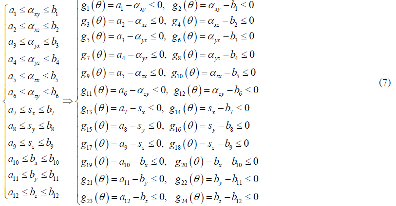
The error function E(θ)of accelerometer is used as it is as an objective function.
And θ are the calibration parameters to be found and expressed as follows.

From this, when the initial point θ1 is obtained using genetic algorithm, the problem of quadratic programming is established as follows to select the optimal direction S from the set of allowable search direction vectors.
min: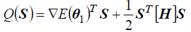
where [H] is a positive matrix that is given as a unit matrix at the beginning. And it is updated in the course of iteration so that it may converge into Hessian matrix of Lagrange function.
The constant  is a number that is taken to prevent the limited region from being separated completely from the admissible region.
Search direction is 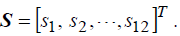
KKT theorem is used to solve this problem.
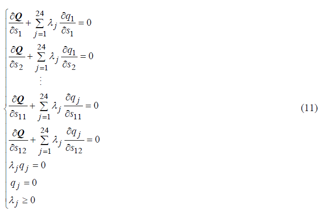
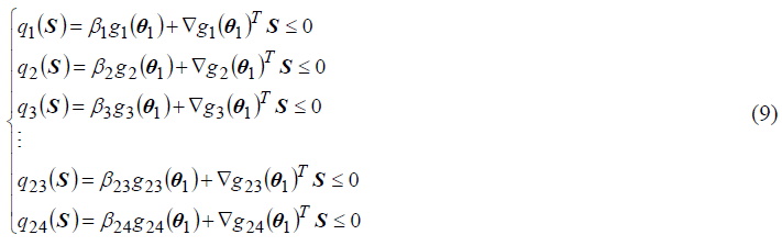
j=1,2,...,24
The solution of this problem is the search direction S and Lagrange multiplier λ1,λ2,....λ24.
Step 2: Search for step size using penalty function method of one variable
In case that the optimal direction is determined in the set of admissible direction vectors, the optimization problem to select the most reasonable step size within the admissible region is referred to the following problem of unconditional extreme value.

where
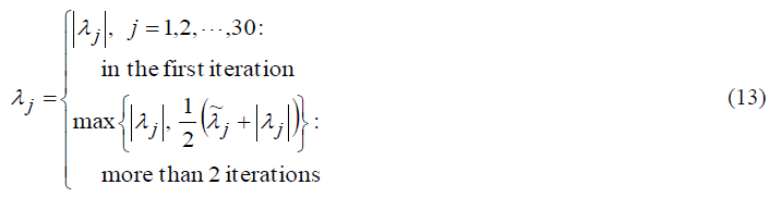
λj is the value of λj that was set in the previousiteration stage
In order to find θ2 , let

If Eq. (14) is put into Eq. (12),

Since the problem of extreme value is that of one variable with respect to step size α, the step size α can be determined easily.
Step 3: Update of Hessian matrix by BFGS method Hessian matrix uses BFGS method in the sequence quadratic programming and according to this method Hessian matrix is updated in each step size as follows.
First, Lagrange function is found from 30 limit conditions and objective function.

where E(θ) an objective is function for calibration and gj(θ) is calibration parameter definitions.
Meanwhile,

where 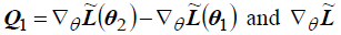 is as follows.
where P1=θ2-θ1.
Therefore, Hessian matrix is updated as follows.
Using the same method, θ3 is computed from θ2 .
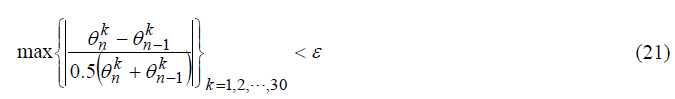
Iteration method is stopped when the convergence criteria are satisfied.
where θkn is the kth element of θn and ε is the threshold, which is used to evaluate the correctness of calibration.
The optimization criteria ε are set to 10-15.
Orientation measurement
Once the auto-calibration procedure has been completed, we can compute the orientation using the accelerometer outputs.
The MEMS IMU is fixed on North-East-Down (NED) frame.
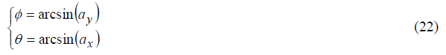
From the accelerations measured through (3) the roll and pitch angles, φ and θ can be estimated by means of the following equations [2]:
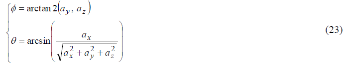
Eq. (22) are frequently used with bi-axial accelerometers, but they suffer from a critical drawback:
The accuracy of the estimated φ and θ depends only on the values of φ and θ.
To overcome this problem, the following trigonometric equations are used here to compute the φ and θ.
Experiments Setup
To verify the effectiveness of the proposed approach, MEMS IMU has been installed on a precision 3-axis turntable.
The output of the MEMS accelerometer is calibrated using different methods. With these outputs orientations are determined and then they are compared with the angles that are set on the precision 3-axis turntable.
FIG. 4 shows the device that was used in experimental equipment.

Figure 4: Experimental equipment.
All comparisons are obtained on the MATLAB 2013b software on a TOSHIBA laptop with a CPU of i3-380M.
The turntable outputs the rotation angle with a repetitive positioning accuracy of 0.5° and it is used as reference angles for attitude in this experiments.
Setting range about the pitch and roll angles using turntable are -90°~ +90°, respectively and setting range about the roll is 0°~360°. For the static calibration of the accelerometer, we applied the proposed algorithm to the 3-axis accelerometer in MPU 9250 IMU (See FIG. 5).

Figure 5: MPU 9250 IMU
The IMU that was used in the experiment is MPU9250IMU in which 3-axis accelerometer, 3-axis gyro and 3-axis magnetometer are embedded.
TABLE 1 shows the technical specifications of MPU 9250 IMU.
TABLE 1. Main parameters of 3-axis accelerometer in MPU 9250 IMU.
| Parameter | Conditions | Typ | Units |
|---|---|---|---|
| Measurement range | AFS_SEL=0 | ±2 | g |
| Nonlinearity | Best Fit Straight Line | ±0.5 | % |
| Sensitivity Scale Factor | AFS_SEL=0 | 16384 | LSB/g |
| Cross-Axis Sensitivity | ±2 | % | |
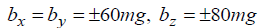
| Zero-G Initial Calibration Tolerance | Component-level, X,Y | ±60 | mg |
| Component-level, Z | ±80 | mg | |
| Zero-G Level Change vs. Temperature | -40°C to +85°C | ±1.5 | mg/°C |
MPU 9250 IMU has been installed in a housing of duralumin and collected the sensor data in I2C mode.
The microprocessor is STM32F407.
To remove the drift according to the temperature change we first designed a thermostat.
Micro-controller processes the measurements from the IMU and sends the result to the host computer through USB-232 converter.
The host computer performs calibration using these measurements.
The sensor data is obtained in 23 different positions for 15 seconds.
Sampling period is 15ms and measuring range is set to ±2g .
Experiments and Results
Static experiments
FIG. 6 shows the calibration result of the accelerometer in 30 different positions. In the figure the green line is the size of reference value (g 1 ), the blue line shows the size of static acceleration before calibration and the red one is the size of static acceleration after calibration.

Figure 6: Typical results for accelerometer calibration.
As shown in FIG. 6, the norm of the 3-axis acceleration measurements does not reach the ideal 1g in the static positions before calibration.
In the experiment, we calibrated the accelerometer using the proposed approach and compared the result with the previous calibration approaches.
The comparison results of hybrid genetic algorithm, Newton’s method and LM method are given in TABLE 2.
TABLE 2. Comparison results of calibration.
| Coefficients | HGA | Newton’s | LM |
|---|---|---|---|
| αxy | 0.016417 | -0.00333 | 0.001921 |
| αxz | -0.104562 | -0.007933 | -0.00124 |
| αyx | -0.030346 | -0.007102 | -0.001734 |
| αyz | 0.106299 | 0.007993 | 0.001228 |
| αzx | 0.034101 | 0.007665 | 0.00172 |
| αzy | -0.013885 | 0.003657 | -0.00196 |
| Sx | 0.961258 | 0.992782 | 0.990739 |
| Sy | 0.948658 | 0.988344 | 1.000908 |
| Sz | 0.964754 | 0.931339 | 0.984876 |
| Ox | 0.001229 | 0.030243 | 0.022078 |
| Oy | 0.028684 | 0.0113 | 0.020588 |
| Oz | -0.0122408 | -0.056756 | -0.00028 |
| Errors after calibration | 2.67E-06 | 3.16E-05 | 4.29E-05 |
From the datasheet of MPU 9250, the values for the initial tolerance of biases are given as:
As seen in TABLE 2, when the Hybrid Genetic Algorithm (HGA) is used, the error are much less than other approaches, and all the obtained estimated values are within this range of initial tolerance.
We simulated the proposed problem using the hybrid genetic algorithm and compared the result with that of the preceding calibration approaches.
TABLE 2 shows the comparison results of calibration when Newton’s method, LM and HGA are used.
To evaluate the accuracy of calibration, the data is obtained in any static attitude for 1 minute and then the distance error of the obtained sensor data after calibrations are analyzed using Newton’s method, LM method and HGA.
The distance error at every time is computed using the following equation.

where SX,SY,SZ are the distance errors in the directions of X,Y,Z axes, respectively.
FIG. 7 shows the distance errors when the different calibration approaches are used.

Figure 7: Comparison of the distance errors after calibration.
As shown in FIG. 7, the distance errors are 6 m, 5.05 m and 3.29 m respectively, and the distance error is the smallest when the hybrid genetic algorithm is used.
Orientation Measurement Experiments
Using the calibrated accelerometer, the roll and pitch angles can be measured in the static status.
We calibrated the navigation device on the 3-axis turntable using Newton’s method, LM method and HGA and compared the measurement result of angles.
The navigation device is installed according to NED frame, the set values of roll and pitch angles are given by rotating the turntable and they are compared with the computation result of attitude that is obtained with the measurement values of accelerometer.
The curves are shown in FIG. 8 and FIG. 9 with the set values of roll and pitch angles taken as +10° and -10° after data filtering.

Figure 8: Computation result of roll angle.

Figure 9: Computation result of pitch angle .
As can be seen from the figures, when HGA is used for calibration, the orientation error is less than 0.15° and the accuracy is much higher compared with the other two approaches.
Even when the experiment is done with the set values of orientation increased or decreased by 10°, the accuracy by HGA is higher than by other two approaches.
Conclusion
In the paper we described the static calibration of MEMS accelerometer using hybrid genetic algorithm.
Using genetic algorithm, we verified the initial values of scale factor and zero bias ones.
Taking these as the initial values of the SQP, we found the optimal solution.
We proved the effectiveness of the calibration using the measurements of MPU 9250 IMU in the stationary position.
The experimental result showed that the navigation error was less when the calibration is done using hybrid genetic algorithm than when the other two approaches are used.
The calibration approach proposed in this paper can be used in the static calibration of gyros magnetometer.
When the accelerometers, gyros and magnetometers are calibrated using this approach, the computation accuracy of attitude can be increased in AHRS.
REFERENCES
- Šipoš M. Improvement of Inertial Navigation System Accuracy Using Alternative Sensors (Doctoral dissertation, Czech Technical University). 2015.
[Google Scholar] [Crossref]
- I. Frosio and S. Stuani. Auto-calibration of a MEMS accelerometer, IMTC 2006-Instrumentation and Measurement Technology Conference, Italy, 2006:519-23. [Google Scholar] [Crossref]
- Skog I, Händel P. Calibration of a MEMS inertial measurement unit. InXVII IMEKO world congress 2006:1-6
[Google Scholar] [Crossref]
- Marinov M, Petrov Z. A static calibration of mems 3-axis accelerometer using a genetic algorithm. Zeszyty Naukowe. Transport/Politechnika Śląska. 2019.
[Google Scholar] [Crossref]
- Xiaoming Z, Guobin C, Jie L, et al. Calibration of triaxial MEMS vector field measurement system. IET Sci. Meas. Technol . 2014;8(6):601-9.
- Fong WT, Ong SK, Nee AY. Methods for in-field user calibration of an inertial measurement unit without external equipment. Meas. Sci. technol. 2008;19(8):085202.
- Syed ZF, Aggarwal P, Goodall C, et al. A new multi-position calibration method for MEMS inertial navigation systems. Meas. sci. technol. 2007;18(7):1897.
- Won SH, Golnaraghi F. A triaxial accelerometer calibration method using a mathematical model. IEEE trans. instrum. meas. 2009;59(8):2144-53.
- Mayagoitia RE, Nene AV, Veltink PH. Accelerometer and rate gyroscope measurement of kinematics: an inexpensive alternative to optical motion analysis systems. J. biomech. 2002;35(4):537-42.
- Tedaldi D. IMU calibration without mechanical equipment.(Calibrazione di IMU svincolata da apparati meccanici).
[Google Scholar] [Crossref]
- Xu X, Tian X, Zhou L, et al. A decision-tree based multiple-model UKF for attitude estimation using low-cost MEMS MARG sensor arrays. Measurement. 2019;135:355-67.