Research

, Volume: 13( 3)

• View PDF
• Download PDF

Implications of Radio Telescope Antenna through 3D Radiation Pattern

*Correspondence:

Debojyoti HalderDepartment of Physics, Rishi Bankim Chandra Evening College, Naihati, West Bengal, India; E-mail: debojyoti_halder@rbcec.in

Abstract

Radio telescopes are based on the basic principle of optical telescopes called the “optical seeing”, where the astronomical object is viewed through a combination of lenses. Unlike optical telescopes, radio telescopes use antennae as the viewing instrument. The wavelength is in radio spectrum and moreover an image is also not formed for seeing. Thus, the radio telescopes may be said to use the principle of “indirect seeing”, which means, after the signals from the radio source in the sky are received using the antenna, they are processed involving electronics and co mputers thereby developing an image using pseudo color which can be seen with the human eye. The prime instrument of a radio telescope is the antenna. Based on the performance of the antenna, the quality of the image is justified. The purpose of this paper is to focus some critical concepts of antenna theories from the engineering point of view, essential for successful operation of the radio telescopes. A basic unit of radiation may be developed to describe the dependence of all the variables involved in r adiation. This unit is called brightness in astronomy. If the brightness is known, then it may be used to calculate the received spectral power etc. on the Earth. In this paper, the relationship between the brightness of the sky and the received power is c ritically examined, particularly when using a radio telescope antenna. The attenuation for the electromagnetic waves passing through an absorbing medium is also considered briefly and the limitations are discussed discussed.

Keywords

Radio telescope; Anten na; Hal Half-wave dipole antenna; Radiation pattern

Introduction

For a linearly polarized antenna like the half-wave dipole, the E-plane pattern is termed as “a plane containing the electric field vector and the direction of maximum radiation” and the H-plane as “a plane containing the magnetic field vector and the direction of maximum radiation”. Since the patterns of the antennae are not uniform over angle of radiation, even if we take a lobe, we find that the power radiated by the lobe at different angles within the lobe is not constant. The antenna reciprocity theorem can be considered to some extent as the theorem has a very important role towards an actual radio telescope. The reciprocity theorem is stated as “If an emf is applied to the terminals of an antenna 1 and the current is measured at the terminals of an antenna 2, then an equal current in both amplitude and phase will be obtained at the terminals of antenna 1 if the same emf is applied to the terminals of antenna 2”. The implications of the reciprocity theorem that are important to be considered for radio telescope antennae are as follows: (a) The radiation pattern of an antenna is unchanged whether used as a receiver or transmitter. Therefore, radiation patterns of the radio telescope antenna-feeds can be measured in the transmitting mode or in the receiving mode inside anechoic chamber. (b) The impedance of an antenna does not change whether used in transmitting mode or in receiving mode. The impedance of the radio astronomical antenna-feeds can be measured inside anechoic chamber in the transmitting mode by measuring the voltage and current at its terminals [1-2]. The detector used for collecting the radiation is an antenna generally called “radio telescope”. Under such circumstances, the equations derived so far have to be modified with the radiation pattern of the antenna. Radio astronomy uses antennas as telescopes. There exists a relationship between the brightness of the source, the temperature of the source (if it is a blackbody) and the output of the antenna seeing or pointing to the source.

Materials and Methods

In practice the radiated power from an antenna does not possess the same strength in all directions, i.e., the strength is more in any particular direction and less or null in some other directions. The energy radiated in a particular direction is measured in terms of field strength or flux density at a point which is fixed radial distance from the center of the antenna. Usually, the performance of an antenna is described in terms of principal E-plane and H-plane radiation patterns [3]. For a linearly polarized antenna like the half wave dipole, the E-plane pattern is termed as “a plane containing the electric field vector and the direction of maximum radiation” and the H-plane as “a plane containing the magnetic field vector and the direction of maximum radiation”. Thus, it is a normal procedure to orient the antennas in such a way that at least one of its principal plane patterns coincide with one geometrical plane as shown in Figure 1.

FIG. 1. Different lobes of a radiation pattern with main lobe oriented with an axis. (a) A 3D view of a radiation pattern. (b)A 2D view of the same radiation pattern. (c) The radiation pattern plotted as a function of angle in one plane.

If we place an antenna at the center of a three-dimensional coordinate system as shown in Figure 2, the electric field, magnetic field and the power per unit all are functions of θ and Φ. The electric field will have two components Eθ (θ, φ) and Eφ (θ, φ) as shown. Similarly, the radiated power will be in the direction of the Poynting vector.

FIG.2. A 3D radiation pattern with its direction of maximum radiation aligned with the z-axis. The electric field components and the poynting vector are shown.

Since the patterns of the antennae are not uniform over angle of radiation, even if we take a lobe, we find that the power radiated by the lobe at different angles within the lobe is not constant. Thus, it is important to define the beam solid angle of an antenna. We consider a practical radiation pattern of the type shown in Figure 3a. As we can see the power is radiated in various directions with different intensities (power per unit solid angle). In Figure 3b, we consider a fictitious radiation pattern having a solid angle ΩA radiating at uniform intensity over this solid angle. If the power radiated using both these patterns are same, the solid angle ΩA is called the “beam solid angle”. Figure 3c shows a two-dimensional comparison between the two patterns. Note that the fictitious pattern showing beam solid angle radiates at the peak intensity of the actual pattern. Similar analogies can be made for individual lobes of the radiation pattern.

FIG. 3. Comparison between actual radiation pattern and the radiation pattern developed from the concept of beam solid angle. (a) A practical radiation pattern. (b) A fictitious beam pattern for calculating the beam solid angle. (c) A comparison between the two patterns in a 2D plane.

Reciprocity theorem and its implications towards radio telescope

The antenna reciprocity theorem can be considered to some extent as the theorem has a very important role towards an actual radio telescope. The reciprocity theorem is stated as “If an E.M.F. is applied to the terminals of an antenna 1 and the current is measured at the terminals of an antenna 2, then an equal current in both amplitude and phase will be obtained at the terminals of antenna 1 if the same E.M.F. is applied to the terminals of antenna 2”. Figure 4 shows the test setup for this theorem. The condition for theorem to be valid is that impedance of the signal generator and the load across the antenna 2 should be zero. Since practically there is no signal generator having zero impedance, it is therefore necessary for both the impedances of the signal generator and the load to be identical [4]. The impedances of the voltmeter and the ammeter are respectively assumed to be infinite and zero. It is also assumed that the frequency of transmission and reception are identical.

FIG. 4. Test setup for verifying the reciprocity theorem.

The implications of the reciprocity theorem that are important to be considered for radio telescope antennae are as follows: (i) The radiation pattern of an antenna is unchanged whether used as a receiver or transmitter. Therefore, radiation patterns of the radio telescope antenna-feeds can be measured in the transmitting mode or in the receiving mode inside anechoic chamber. (ii) The impedance of an antenna does not change whether used in transmitting mode or in receiving mode. The impedance of the radio astronomical antenna-feeds can be measured inside anechoic chamber in the transmitting mode by measuring the voltage and current at its terminals. However, there is a practical limitation of the reciprocity theorem. The theorem fails to be true only when the propagation of the radio waves is highly affected by the presence of the Earth’s magnetic field and disturbances created in the ionosphere.

Analysis of a half wave dipole antenna

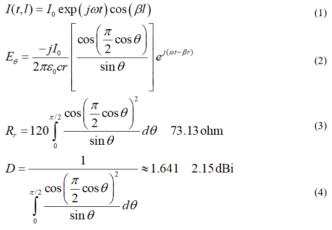
A standing wave pattern is formed if the dipole is excited at a frequency corresponding to the wavelength λ. The current distribution across the antenna length is shown in the figure. Let l be an axis along the dipole such that at l=0, the current I is maximum, i.e., I=I0 and at l=λ/2. If the angular frequency of the sinusoidal signal be ω, then the current distribution I (t, l) across the dipole length as a function of time t can be expressed as in Eqn. 1, where β=2π/λ. The electric field at a very large distance r from the center of the dipole is expressed as in Eqn. 2, where c is the velocity of light and ε0 is the permittivity of free space. The electric field distributions are shown in E-plane and H-planes. The E-plane is a plane aligned along the axis of the dipole and hence can be rotated along the dipole axis. The radiation resistance is expressed in Eqn. 3. This however is s not enough to characterize the dipole impedance, as there is also an imaginary part. Hence, it is better to measure the impedance [5]. The directivity is expressed in Eqn. 4 which comes to nearly 2.15 dBi.

The half wave dipole antenna, one of the most common antennae, is formed from two quarter wavelength conductors or elements placed back-to-back for a total length of λ/2 as shown in Figure 5a, where λ is the wavelength. The quantity within the third bracket ‘[ ]’ of Eqn. 2 behaves slightly different from sin θ which is shown by dotted lines in Figure 5b.

FIG.5. Analysis of a dipole. (a) Current distribution on the dipole due to excitation from a source. (b) Behaves slightly different as shown by dotted lines.

Relationship between the received power and ‘brightness of the sky’

Let an electromagnetic radiation possessing infinitesimal bandwidth dν Hz generated from a region of the sky is falling on a flat area A on the surface of the Earth as shown in Figure 6.

FIG. 6. Radiation falling on the surface of the Earth from a portion the sky with brightness B and forming a solid angle dΩ and incident at angles of θ and Φ respectively with z-axis and x-axis.

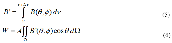
The variation of brightness B as a function of frequency is known as “brightness spectrum”. Integrating B over a bandwidth Δν Hz, gives the total brightness B’ within this frequency band as expressed in Eqn. 5. If this integration is performed over the entire radio spectrum range, the “total radio brightness” is obtained. In view of total radio brightness B’, we can express the received power W over a bandwidth Δν and solid angle Ω as in Eqn. 6. Note that B’ is also a function of angle of incidence, i.e., θ and ?.

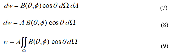
The power per unit bandwidth is called as “spectral power” dω and is measured in watts Hz-1. The spectral power dω may be re expressed as in Eqn. 7. Since for a distant source dw is independent of the position of dA on the surface A, the total spectral power received on the surface A can be expressed as in Eqn. 4. By integrating Eqn. 8, we can achieve the spectral power from a solid angle Ω as expressed in Eqn. 9, where, w is the spectral power in watts Hz-1.

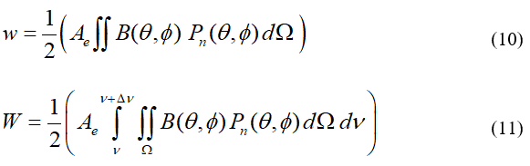
The detector used for collecting the radiation is an antenna generally called “radio telescope”. Under such circumstances, the equations derived so far have to be modified with the radiation pattern of the antenna [6,7]. Let an antenna having an effective aperture Ae and a normalized response pattern Pn(θ,φ) be used for receiving the radiations from the sky. Then Eqn.9 can be modified to produce Eqn. 6, where Ae is in m2. Note that limits of Ω should be selected such that the integration does not miss the nonzero points of the antenna response Pn(θ,φ). Also to be noted that, a factor of half has been introduced in Eqn. 10 considering the antenna responds to only one polarization of the incoming radiation thereby receiving only half of the power. Thus, the total power received by a radio telescope antenna can be expressed as in Eqn. 11.

Effects of absorption and emission of electromagnetic waves

When an electromagnetic wave travels through free space, the flux density decreases with the square of distance called the “inverse square law”. If the source is distant, then within a small region situated much away from the source, the change in flux density is negligible because the waves are almost parallel [8]. However, if the space is filled with gas containing absorbing elements enclosing this small region, then the flux density decreases as the waves propagate through this medium. In Figure 7, we have illustrated this considering a small region of length x along the direction of propagation.

Radio astronomy uses antennas as telescopes. There exists a relationship between the brightness of the source, the temperature of the source (if it is a blackbody) and the output of the antenna seeing or pointing to the source.

FIG. 7. Attenuation of the electromagnetic waves passing through an absorbing medium.

Results and Discussion

The antenna is usually polarized, i.e., at a large distance from an antenna, the electric field vector in the radiated field at any given time lies in one plane parallel to the direction of propagation. The magnetic field remains perpendicular to the electric field. As the wave progresses in its travel through space the electric field (and the magnetic field) may

• Continue to lie in the same plane or
• Change its orientation within each wavelength traveled.

For the former case, the wave is said to linearly polarized while in the latter case, the wave could be circularly or elliptically polarized depending on the whether the amplitude of the electric field remain fixed or change with angle respectively. The circular or elliptical polarizations can again be classified as left circular/elliptical or right circular/elliptical depending on the directions in which the plane of polarization rotates. The dipole type antennae are linearly polarized whereas helical antennae are circularly polarized [9-12].

Astronomical radio sources have the possibility of all type of polarizations, viz. linearly polarized, elliptically polarized, circularly polarized, unpolarized or a combination of unpolarized with the remaining types. It is important to obtain the complete information of the astronomical source which is possible by using two linearly polarized antennae with their planes of polarization perpendicular to each other or two circularly polarized antennae having opposite polarizations, viz. left circular and right circular. If an antenna having only one polarization is used for receiving the signals from an unpolarized astronomical source, the antenna can capture only half of the flux density produced by the source. This is because an unpolarized source can be thought of as two independent (incoherent) noise sources of equal strength connected to two linearly polarized antennae with the angle between the plane of polarizations of the two antennae kept as 90°. Two circularly polarized antennae, one left circularly polarized and the other right circularly polarized can also be used instead of the two linearly polarized antennae. Thus, in order to absorb the entire flux density at the aperture, two antennae are required with properly aligned polarization planes [13-16]. So far, we have considered a lossless antenna, though in reality every antenna incorporates losses of its own which contribute to the system temperature. These losses contribute to some noise in the received antenna signal. If the signal received is less than this noise, it cannot be detected. Moreover, radio telescope antennas are connected to receivers for amplifying and further processing the signals received from radio sources. The first stage of a receiver system is usually a low noise amplifier which does a major contribution to the noise from the receiver end. Thus the “minimum detectable signal” using the antenna is further lowered. There are also contributions of noise by the cable connecting the antenna with the low noise amplifier [17,18]. The radio telescope system as a whole can be viewed as a combination of: (a) Antenna; (b) Transmission line and a receiver whose noise is slightly more than the contribution by the low noise amplifier. Due to this combination, a noise is visible at the terminals of the antenna. If the temperature received by the antenna is lower than this noise temperature of the system which is known as “system temperature”, the radio telescope will fail to detect the temperature of the remote source. Every radio telescope is limited to a minimum detectable temperature. The minimum temperature that a radio telescope can successfully detect is restricted by the fluctuations at the receiver output. These fluctuations are due to random nature of the noise whose value is proportional to the system temperature Tsys of the radio telescope [19]. The system temperature Tsys is principally dependent on two:

• Contribution from the antenna temperature TA.
• Contribution from the receiver temperature TR.

In theory it is possible to reduce the system noise to any extent by

• Increasing the time of integration after detection.
• Increasing the pre-detection bandwidth or by.
• Taking the mean values of more than one observation.

However, in reality it is not possible to increase the integration beyond a point where it starts distorting the true profile of a radio source. Similarly, the bandwidth cannot be made too wide for it will result in

• Loss of spectral information.
• Increase in local interference from terrestrial sources.

Conclusion

In conclusion, the study of radio telescope antennas through 3D radiation patterns offers critical insights into the antenna's performance and its ability to capture radio waves from distant sources. By visualizing the radiation pattern in three dimensions, researchers can optimize antenna design, improve signal reception, and enhance the accuracy of astronomical observations. This approach helps in addressing challenges like interference and noise, ultimately advancing the field of radio astronomy. The use of 3D patterns is instrumental in ensuring the precision and efficiency of radio telescopes in various scientific applications.

References

1. Joardar S, Bhattacharya AB. Simultaneous resolving of frequency separated narrow band terrestrial radio sources by multi antenna spectrum monitoring systems assisting radio astronomy. J Electromagn Waves Appl. 2006;20(9):1195-1209.

   [Crossref] [Google Scholar]

2. Joardar S, Bhattacharya AB. Two new ultra wideband dual polarized antenna-feeds using planar log periodic antenna and innovative frequency independent reflectors. J Electromagn Waves Appl. 2006;20(11):1465-1479.

   [Crossref] [Google Scholar]

3. Olsson R, Kildal PS, Weinreb S. The Eleven antenna: A compact low-profile decade bandwidth dual polarized feed for reflector antennas. IEEE Trans Antennas Propag. 2006;54(2):368-375.

   [Crossref] [Google Scholar]

4. Best SR. Distance-measurement error associated with antenna phase-center displacement in time-reference radio positioning systems. IEEE Antennas Propag Mag. 2004;46(2):13-22.

   [Crossref] [Google Scholar]

5. Rao S, Wilton D, Glisson A. Electromagnetic scattering by surfaces of arbitrary shape. IEEE Trans Antennas Propag.1982;30(3):409-418.

   [Crossref] [Google Scholar]

6. Joardar S, Bhattacharya AB. Uniform gain powerspectrum antenna-pattern theorem and its possible applications. Prog Electromagn Res. 2007;77:97-110.

   [Google Scholar]

7. Seo DK, Kim KT, Choi IS, et al. Wideangle radar target recognition with subclass concept. Prog Electromagn Res. 2004;44:231-248.

   [Google Scholar]

8. Joardar S, Bhattacharya AB. Algorithms for categoric analysis of interference in low frequency radio astronomy. J Electromagn Waves Appl. 2007;21(4):441-456.

   [Crossref] [Google Scholar]

9. Joardar S, Bhattacharya AB. Uniform gain powerspectrum antenna-pattern theorem and its possible applications. Prog Electromagn Res. 2007;77:97-110.

   [Crossref] [Google Scholar]

10. Kitchin C. Astrophysical techniques(Book). Adam Hilger, Ltd., Bristol, England, 1984:451.

    [Crossref] [Google Scholar]

11. Joardar S, Bhattacharya AB, Bhattacharya R. Astronomy and Astrophysics. Jones and Bartlett Learning; 2008.
12. Joardar S, Bhattacharya A. A novel method for testing ultra wideband antenna-feeds on radio telescope dish antennas. Prog Electromagn Res. 2008;81:41-59.

    [Crossref] [Google Scholar]

13. Birney DS, Gonzalez G, Oesper D. Observational astronomy. Cambridge University Press, United Kingdom. 2006.
14. Kreysa E, Gem