Original Article

, Volume: 5( 1)

• View PDF
• Download PDF

Qualitative Analysis and Asymptotics of Solutions of the Gkp-Class Equations with Variable Dispersion

*Correspondence:

Belashov VYU, Kazan (Volga Region), Federal University, Kazan, Russia, Tel: +86-27-67863760, E-mail: davymanyika@yahoo.com

Abstract

In this paper we study the dynamical systems associated with the generalized Kadomtsev-Petviashvili (GKP) equation with variable dispersion and consider the structure of possible multidi-mensional solutions and their asymptotics. We also present some considerations on constructing of the phase portraits of the systems in the 8-dimensional phase space for the GKP equation on the basis of the results of qualitative analysis of the generalized equations of the KdV-class.

Keywords

dynamical system; generalized KdV equation; GKP equation; multidimensional solutions; phase space; qualitative analysis; solitons; structure of solutions; variable dispersion

Introduction

Basic equations

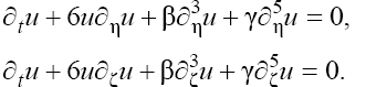
Consider the generalized Kadomtsev-Petviashvili (GKP) equation (or so-called Belashov-Karpman (BK) [1-3] equation without the terms describing the dissipation and instability):

(1)

Where and are the transverse coordinates. At Eq. (1) is the classic Kadomtsev-Petviashvili (KP) equation which is the completely integrable Hamiltonian system and has in case the solutions in form of the 1D (for βκ < 0 ) or 2D (for βκ > 0 ) solitons [4,5]. The structure and the dynamics of the solutions of the non-integrable analytically GKP model (1) with β, γ = const has been investigated in detail in Dynamics of two-dimensional solitons in weakly dispersive media [1,2] where it was shown that in dependence on the signs of coefficients β, γ and k the 2D and 3D soliton type solutions with the monotonous or oscil-latory asymptotics can take place. In Radiophysics and quantum electronics [6] the asymptotes of the 1D analogue of Eq. (1) with were studied, and the sufficiently complete classification of its 1D solutions in the phase space was constructed.

Note, that if the dispersion in medium is variable, introducing the high order dispersive correction (term with γ ) into the KP equation has a principal role. Thus, for example, in the problems of the propagation of the 2D gravity and gravity-capillar waves on the surface of "shallow" water [3] when β is defined respectively as and where H is the depth, ρ is the density, and σ is the coefficient of surface tension of fluid, the depth can be variable, H = H(t, x, y) , and in this case β also becomes the function of the coordinates and time. Similar situation takes place on studying of the evolution of the 3D fast magneto-sonic (FMS) waves in a magnetized plasma in case of the inhomogeneous and/or non-stationary plasma and magnetic field [7,8] when β is a function of the Alfvén velocity

In these cases the situations, when or even becomes equal zero are possible, that, however, does not mean that the dispersion in medium is completely absent, simply it is necessary to keep the next order dispersive term in the Taylor expansion of a full dispersion equation with respect to k, at this, a balance between nonlinearity and dispersion, defining the existence of the soliton, will be conserved, and the term proportional to the fifth derivative will appear in the KP equation. Therefore, if the dispersion can vary in medium, it is necessary to consider the BK equation in form (1), namely the GKP equation.

So, our purpose is the generalization of the results obtained in Radiophysics and quantum electronics [6] to the multidimensional cases when β or/and γ are not constants (the dispersion is variable) with due account of the results presented in [3,4].

To avoid unnecessary cumbersome expressions, consider Eq. (1) in the 2D form assuming that . Further generalization of the technique used (as well as the results obtained) to the full 3D case is rather trivial, as we demonstrate below. Assume that and, for clarity, (the latter can be easily obtained by the scale transform in the GKP equation).

Now, let us introduce the new variables: 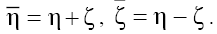Applying first and then to (1) we obtain the pair of one-dimensional equations:

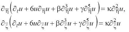(2)

written in the reference frame with the axes and rotated through an angle +45? relative to the axes and

Representation (2) means in fact that the starting Eq. (1) admits two types of 1D solutions, and satisfying the first and the second equations of the set (2), respectively. It is necessary, however, to bear in mind that the "onedimensionality" of these solutions nevertheless implicity assumes the linear dependence of each of the new variables and on both coordinates, and

Integrating Eqs. (2) over and , respectively, we obtain equiform generalized KdV equations

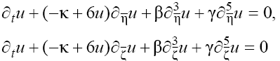(3)

coupled with each other by the way of the change of the coordinates made above. Now, transferring to the coordinates moving along the corresponding axis with the velocity applying the change 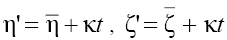in Eqs. (3) and omitting “primes” for simplicity, we write Eqs. (3) in the standard form:

(4)

So, we can now conduct the analysis for only one generalized equation of the set (3), and then, making the inverse change of the variables, extend the results to the 2D solutions of the GKP equation (1) with

Qualitative analysis for 1D equation

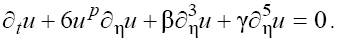
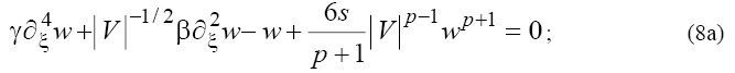
Taking into account the more general case we extend the class of Eqs. (4) by introducing the arbitrary positive exponent p of the nonlinear term:

(5)

Equation (5) for is the usual KdV equation when p =1, and it is the modified KdV (MKdV) equation when p=2. The asymptotics of (5) with p =1 were first investigated in [1,9] where it was shown that depending on the signs of the coefficients β and γ the soliton type solutions with monotonous or oscillating asymptotics can take place. But note, that Eq. (5) with and is not exactly integrable (i.e., the known analytical methods such as the IST method, are not applicable to this equation). In Radiophysics and quantum electronics [6] Eq. (5) was investigated by the methods of the both asymptotic and qualitative analysis, and, as a result, the sufficiently full classification of its solutions was constructed. In this section we mainly follow the ideas and technique of Radiophysics and quantum electronics [6].

Note, that from the physical point of view, the cases when in Eq. (5) p =1,2 are the most interesting, and applications for p >2 are presently unknown. However, since equations of the family (5) with an arbitrary integer p >0 demonstrate, to a considerable extent, similar mathematical properties, we use here a general approach elucidating, apart from other, the dependence of the characteristics of the solutions on the nonlinearity exponent.

Performing transformation and integrating (5) in we obtain:

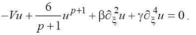(6)

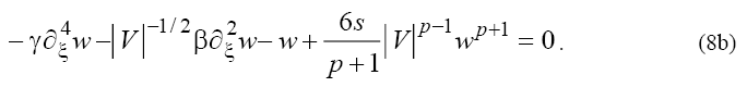
Assuming without loss of generality that and , after the change we convert (6) to

(7)

where

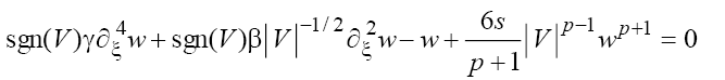
Depending on sign of V in (7) the following two cases can be considered:

However, as one can see from (5), the velocity of the wave, V, depends on the equation’s coefficients and it is restricted by:

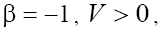The right-hand sides of inequalities (9) correspond to results obtained in [1} and comparing these relations with expressions (8a) and (8b) leads to contradictions in the cases and respectively. Therefore, below we will limited by the consideration of cases (a) with and (b) with and

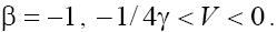
Qualitative analysis and asymptotes of the solutions

First, we note that every equation of the set (8) is equivalent to the set of the first order ordinary differential equations

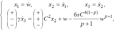(10)

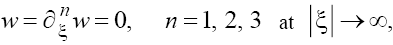
Where the dots stand for the ?-derivatives, and the signs in the brackets correspond to three cases mentioned above; furthermore,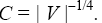 Solutions of Eqs. (10) are stable if there exist the singular trajectories of the imaging point in the phase space 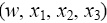of the set (10). Each trajectory of its kind is related to the state of equilibrium near the maximum of the soliton-like solution and at the boundaries Assuming as the boundary conditions that

(11)

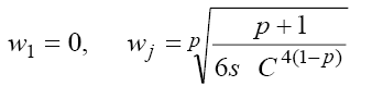
we can find from (10) the number as well as the coordinates of the singular points:

(12)

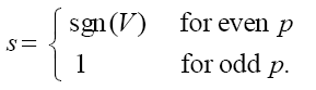
where the points and correspond, respectively, to and the bending points of the function for the odd and j = 2, 3 for the even p, in the last case Considering only real roots of (12) we immediately conclude (using the Sturm’s theorem) that for the odd p there are two singular points, and for any even p there are three singular points. The distance between the singular points defines the amplitude of the soliton-like solution of (6). Besides, the value of the nonlinearity exponent p defines a character of dependence for p >1 this dependence becomes nonlinear ( Figure 1 ) unlike the known linear one for p =1 (e.g., in the case of the KdV equation). As one can see in Figure 1 , for the even p the solutions of Eq. (6) can have the positive as well as negative polarity for any sign of V .

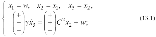
To investigate the types of the singular points, it is necessary to linearize the set (10) in the neighborhood of every point. Using the Taylor’s formula, we obtain from Eqs. (10) [6]:

1) for the singular point that corresponds toin (6), taking into account the conditions (11),

2) for the singular point that corresponds to

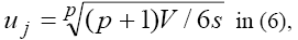
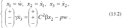
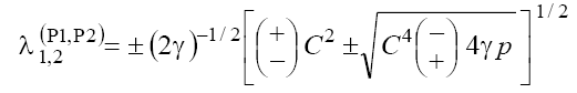
Since the sets (13) are essentially four-dimensional, we investigate them by expanding of the corresponding canonical systems into the subsystems [4]. In this case, it is possible to consider the phase portraits of the linear sets (13) as projections of the singular points and trajectories onto two planes. For singular point we obtain that the eigenvalues of the matrices of subsets of set (13.1) [4] corresponding the phase planes P1(w, x₁) and P2(x₂,x₃) are defined by:

(14)

In the case (a) with 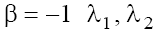are real on the phase plane P1 and pure imaginary on the phase plane P2, besides, on both planes. In the case (b) with taking into account the conditions (9), the characteristic roots and are complex with positive and negative real part on the planes P1 and P2, respectively, and In the case (b) with taking into account condition (9.2), all four roots are real and on both planes. Therefore, the singular points w1= 0 of three types exist in the phase space, namely: the “saddle–center” point, the “stable focus–unstable focus” point, and the “saddle-saddle” point in the cases mentioned above, respectively.

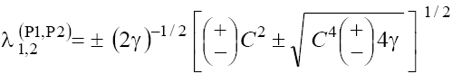
Considering by analogy the matrix of subsets corresponding to set (13.2) we obtain eigenvalues for the singular points w_j defined by (12) in three cases considered for the subsets corresponding to the projections to the phase spaces P1(w, x₁) and P2(x₂, x₃) [6]:

(15)

One can see from (15) that the character of the singular point depends on the nonlinearity exponent p defining the wave velocity 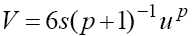. Nevertheless, conditions (9) remain valid and in these cases as well.

Analysis of (15) enables to conclude the following. The eigenvalues and are complex (moreover with the positive real parts on the plane P1 and the negative ones on the plane P2 in case (a) taking into account the condition (9.1). In case (b) with and are real on the plane P1 and pure imaginary on plane P2, and in the both cases. In the case (b) with the situation is analogous to that of the case (b) with Therefore, only singular points wj of the type “stable focus–unstable focus” take place in phase space in the case (a), and of the type “saddle-center” take place in the case (b) for both signs of β.

To study the global phase portraits including singular trajectories corresponding the stable solutions of the Eqs. (10), in Solitary waves in dispersive complex media [4,6] the Bendixon and Dulac criterions have been used, and also the first and the second Lyapunov quantities have been calculated. Omitting here cumbersome mathematical calculations, we note that in all three cases considered the closed trajectories have place in the phase space. At this, formulae (14) and (15) enable us to obtain such parameters of the curves as their directions and, consequently, the angles with respect to the coordinate axes on both planes, and, therefore, to construct the global phase portraits.

The examples of such phase portraits for the cases (a) and (b) for p =1, 2 are shown in Figure 2a and 2b and Figure 3a and 3b.

Using the values of the characteristic roots and (14) for singular points w₁=0, taking into account the conditions (9) and (11) we obtain the asymptotics of the solutions of Eq. (5) for considered cases [4], namely:

1) for the cases (a) and (b) with

(16.1)

(The upper/lower sign corresponds to the cases (a)/(b), respectively);

2) For the case (b) with

Where A₁, A₂ and Θ are arbitrary constants. As we can see from (16), in the solutions of (5) in dependence of the signs of V and β the solitons with both monotonous and oscillating asymptotics can take place. At this, the phase portraits shown in Figure 2a and 2b correspond to the solitons with monotonous asymptotics, and the phase portraits shown in Figure 3a and 3b correspond to solitons with oscillating asymptotics. Figure 2c and 3c show the results of numerical integration of Eq. (5) for the initial condition that corresponds the results of the asymptotic analysis.

Generalization of the results to the BK-class equations

Making the inverse change of the variables, extend the obtained results to the 2D solutions of the GKP equation (1) with The asymptotics of the solutions are defined by relations [3,4]:

(17)

where A₁, A₂ and are the arbitrary constants, and (here the signs "plus" and "minus" relate to the first and second equations of the set (2), respectively). As we can see from (17), (18), solitons with monotonous as well as oscillating asymptotics can take a place depending on the signs of V and β as the solutions of Eq. (1). (Note, that for and any solutions of Eqs. (2) have form and, consequently, also describe a soliton with monotonous asymptotics [3,4].) Figure 4 shows the results of numerical integration of Eq. (1) with the initial condition that confirms the results of our asymptotic analysis.

Other correlations of signs of V and β are not realized [3,4].

As to the proper transform of the phase portraits of the system and "bind" them for the 2D equation, owing to the phase space is 8-dimensional in this case, we can employ the results obtained in [5,6] coupling the characteristics of every singular point of each equation of the set (2) in the 8-dimensional phase space, at this the type of the singularities in the 4-dimensional subspaces [4] under the inverse transform of the coordinates, , is not changed, and only parameters of the phase portraits that correspond to solutions of the same class change (leading to the respective changes such parameters as the amplitude, the fronts steepness, frequency of the oscillations etc) [7-9].

Concluding remarks

To conclude, we note that for the BK equation we considered only the particular cases when it is possible to neglect the effects of dissipation and different types of instability here. For other cases when it is necessary to account dissipation and instabilities, more complex wave structures resulting from the simultaneous presence of all the effects discussed, for example, in Solitary waves in dispersive complex media [4] can be observed. Indeed, results obtained numerically in [10-12], demonstrate that in general BK model [4] with in the presence of the Gaussian random fluctuations of the wave field (for harmonic initial conditions and initial conditions in the form of a solitary pulse) stable wave structures of the soliton-like type can be formed too, with the time evolution. Furthermore, stable soliton structures can be formed also for An analytical study of such cases is highly complicated, however, although the approach considered above can be used for them as well. Note also that the results presented here for the GKP equation can be very useful when studying solutions and interpreting the multidimensional phase portraits of more complicated multidimensional model equations [3,4,13].

References

1. Donald HP. Introduction to high energy physics. Cambridge University Press.2000.
2. Nakamura K. Review of particle physics. Journal of Physics G: Nuclear and Particle Physics. Bibcode. 2010;37
3. Barbier R, Berat C, Besancon M, et al. R-parity violating supersymmetry. Phys. Rept. 2005;420:1
4. Braibant S, Giacomelli G, Spurio M. Particles and fundamental interactions: An introduction to particle physics. Springer. 2009:313-314.
5. Robinson MB, Ali T, Cleaver GB. A simple introduction to particle physics Part II. arXiv:0908.1395[hep-th]. 2009
6. The ‘Higgs boson’.CERN.
7. Amsler C, Doser M, Antonelli M, et al. Particle data group, Phys Lett B. 2008;667:1.
8. Particle Physics and Astrophysics Research.The Henryk Niewodniczanski Institute of Nuclear Physics. 2012.
9. Robinson MB, Bland KR, Cleaver GB, et al. A simple introduction to particle physics. 2008
10. Anderson PW. More is different. Science. New Series, 1972;177:393.
11. Machleidt R.Spin and isospin in nuclear interactions. Adv. Nucl. Phys and references therein. 1989;19:189
12. Seki V, Kolck UV, Savage MJ. Proceedings of the Joint Caltech/INT Workshop: Nuclear Physics with Effective Field Theory, ed.1998.
13. Kaplan DB, Savage MJ. Effective field theory for nuclear physics. Wise Phys. Rev. C59. 1999;617.
14. http://www.hep.anl.gov/ndk/hypertext/nu industry.html
15. Wolfenstein L, Mikheyev SP, Smirnov AY. Sov J NuclPhys.1985;42:913.
16. Fukuda Y. Super-kamiokande collaboration.Phys Rev Lett 81;1998: 1562; IBID. 82;1999:2644; ibid. 82;1999
17. Suzuki Y. Talk at the XIX International Symposium on Lepton and Photon Interactions at High Energies, Stanford University, 1999:914.
18. Bernstein IB, Rabinowitz IN.Theory of electrostatic probes in low-density plasma. AIP Physics of Fluids.1959;2:112-121.
19. Laframboise JG. Theory of spherical and cylindrical Langmuir probes in a collisionless, Maxwellian plasma at rest, Toronto: UTIAS Report No.100 University of Toronto.1966.
20. Bilyk O, Holik M, Pysanenko A, et al.The OML theory for electron collection for gas pressures. Vacuum.2004;76:457.
21. SuditD, Woods R.A study of the accuracy of various Langmuir probe theories.J Appl Phys. 1994;76:4488.
22. Demidov VI, Ratynskaia SV, Rypdal K. Electric probes for plasmas: The link between theory and instrument.Rev SciInstrum.2002;73:3409.
23. Bohm D, Burhop EHS, Massey HSW. The characteristics of electrical discharges in magnetic fields. New York: McGrawHill, New York. 1949.
24. Johnson EO, Malter L.A floating double probe method for measurements in gas discharges. Phys Rev.1950;80:56.
25. Ivanov YA, Lebedev YA, Polak LS. Methods of in situ diagnostics of non-equilibrium plasma-chemistry. Moscow: Nauka. 1981.
26. HoegyWR, Wharton LE.Current to a moving cylindrical electrostatic probe. J Appl Phys. 1973;44:5365.