Original Article
, Volume: 6( 1)On The Stability of Collinear Equilibrium Points in the Relativistic R3BP with a Smaller Oblate Primary
- *Correspondence:
- Nakone B , Department of Mathematics, Faculty of Science, Usmanu Danfodiyo University, Sokoto, Nigeria, Tel: +23470561018; E-mail: bnakone@yahoo.com
Received: November 26, 2016; Accepted: February 08, 2017; Published: February 16, 2017
Citation: Jagadish S, Nakone B. On the Stability of Collinear Equilibrium Points in the Relativistic R3BP with a Smaller Oblate Primary. J Space Explor. 2017;6(1):112.
Abstract
This study investigates the effects of relativistic factor and oblateness of the smaller primary on the locations and stability of collinear points in the framework of the post-Newtonian approximation. The collinear points are found to be unstable. A numerical exploration in this connection, with some members of our solar system reveals that the locations of the collinear points are affected prominently by the relativistic factor in the absence of oblateness and they are also affected significantly by the oblateness factor in the absence of relativistic terms. It is also found that in most of the cases, the position of is negligibly affected by the relativistic and oblateness factors. More specifically, all parameters involved have no effect on the position of of the Sun-Mars system. It is noticed that the oblateness and relativistic factors have same separate effect on the position of of the Sun-Uranus system and have also the same effect on the position of of the Sun-Neptune system. It is also discovered that in the presence of relativistic terms, the effect of oblateness on the Sun-Planet pairs does not show physically as shown from the third and fourth entries.
Keywords
Celestial mechanics; Oblateness; Relativity; R3BP
Introduction
The general three-body problem concerns the motion of three arbitrary spherically symmetric bodies. Each body is modeled as a point mass and their motion is influenced solely by the gravitational forces they exert on one another and also their motion has no specific path. There is no closed form analytical solution to the general three-body problem.
The restricted three-body problem is an approximation of general three-body problem in which one body is assumed to have an infinitesimal mass as compared to the other two bodies each of much larger. The two massive bodies called primaries revolve around their common center of mass in circular orbits in a rotating coordinate system in which the infinitesimal mass can be at rest at five equilibrium points also called equilibrium solutions. Three of them labeled L1, L2, L3 and are called collinear points and they are lying on the line joining the primaries, while the other two labeled L4 and L5 called triangular points form equilateral triangles with the primaries. The triangular points are stable for the mass ratio μ < 0.03852... [1] and the analysis has revealed that the collinear points are unstable in both linear and nonlinear sense.
The equilibrium solutions are very useful for the space mission design. For example the Solar and Heliospheric Observatory (SOHO) and Wilkinson Microwave Anisotropy Probe (WMAP) launched by NASA are in operation at the collinear points L1 and L2 of the Sun-Earth system.
The classical restricted three-body problem considers the bodies to be strictly spherical, but in nature they are either oblate or triaxial. It must be noted that the asphericity of the primaries is of great importance [2,3].
Some important contributions, related to the equilibrium points in the restricted three-body problem with one or both primaries are oblate or triaxial can be found as studied by Sharma and Subba Rao [4]; Oberti and Vienne [5]; Abouelmagd et al.[7]; Singh and Umar [8].
The relativistic restricted three- body problem as we consider it arose from the work of Brumberg [9,10]. Later on, Bhatnagar and Hallan [11], Douskos and Perdios [12] and Ahmed et al. [13] studied the stability of triangular points of the same model problem and obtained three different results regarding the region of stability.
Ragos et al. [14] studied the existence, position, and stability of collinear points of the same model problem. Recently, the study of equilibrium points in the relativistic restricted three- body problem with perturbing forces such as radiation, oblateness and small perturbations in the Coriolis and centrifugal forces has been conducted by several authors (Abd El- Bar and Abd El- Salam [15]; Abd El-Salam and Abd El- Bar [16]; Singh and Bello [17,18]; Katour et al. [19]; Bello and Singh [20].
From authors’ knowledge, no work has been done on the stability of collinear points with perturbing forces in the relativistic R3BP.
Hence, it raised a curiosity in our minds to study the effect of oblateness of the smaller primary on the locations and stability of collinear equilibrium points in the relativistic R3BP.
This paper is organized as follows: In Sect. 2, the equations governing the motion are presented; Sect. 3 describes the positions of collinear points, while their linear stability is analyzed in Sect. 4. A numerical application of these results and discussion are given in Sect.5 and 6, respectively. Finally, Sect. 7 conveys the main findings of this paper.
Equations of motion
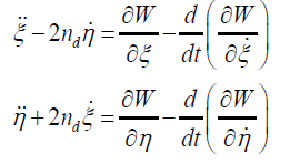
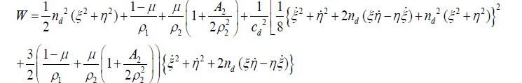
The pertinent equations of motion of an infinitesimal mass in the relativistic R3BP in a barycentric synodic coordinate system and dimensionless variables, when the effect of oblateness of the smaller primary is introduced with the help of the parameter can be written as Brumberg [9] and Bhatnagar and Hallan [11].
 (1)
(1)
With
 (2)
(2)
 (3)
(3)
 (4)
(4)
where  is the ratio of the mass of the smaller primary to the total mass of the primaries, ρ2 and ρ2 are distances of the infinitesimal mass from the bigger and smaller primary, respectively; c is the perturbed mean motion of the primaries; c is the velocity of light.
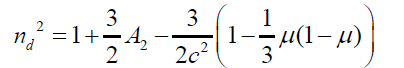
 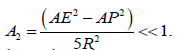 [21], where AE and AP are the equatorial and polar radii of the smaller primary, and R is the
distance between the primaries.
[21], where AE and AP are the equatorial and polar radii of the smaller primary, and R is the
distance between the primaries.
It should be noted here that the second and higher powers of A2 and  have been ignored in writing above equations.
Location of collinear points
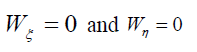
Equilibrium points are those points at which no resultant force acts on the third infinitesimal body. Therefore, if it is placed at any of these points with zero velocity, it will stay there. In fact, all derivatives of the coordinates with respect to the time are zero at these points. Therefore, the equilibrium points are solutions of equations:
 (5)
(5)
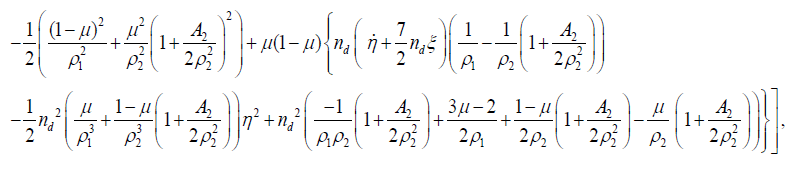
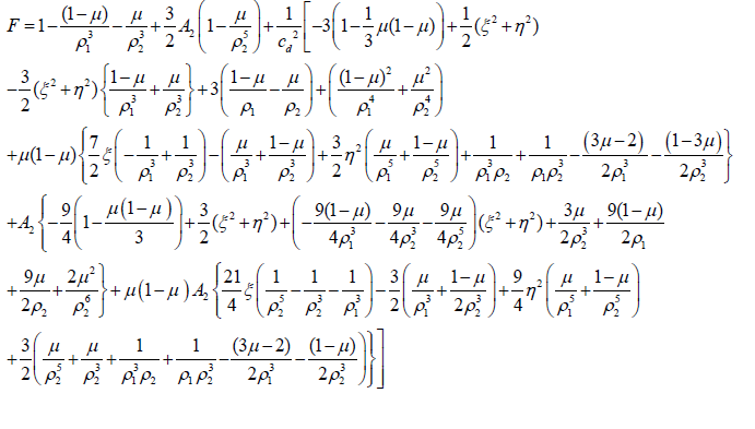
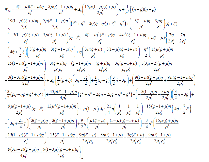
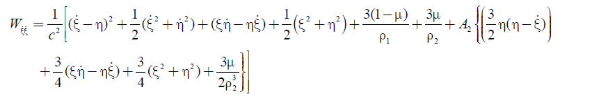
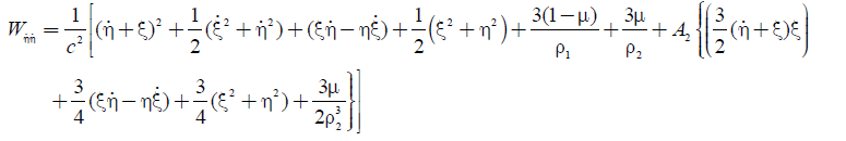
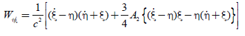
where, Wη and Wη may be written as
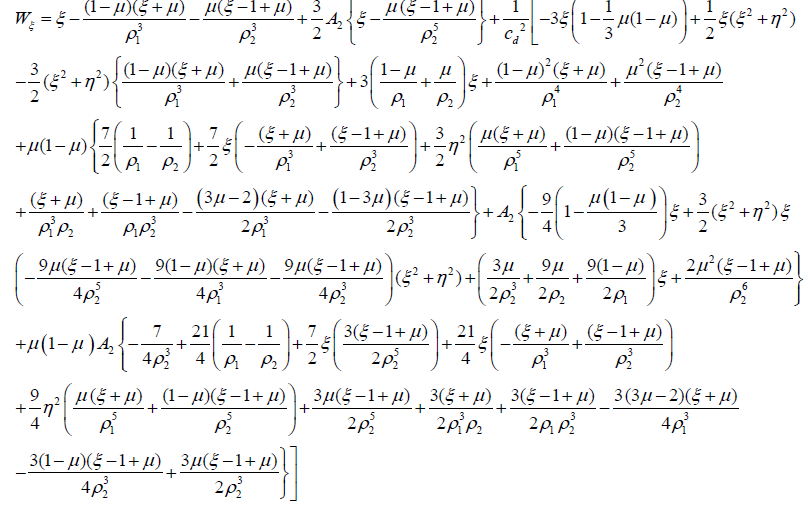
and
Wη= ηF
with
In order to find the collinear points, we put in equation (5). Their abscissae are the roots of the equation
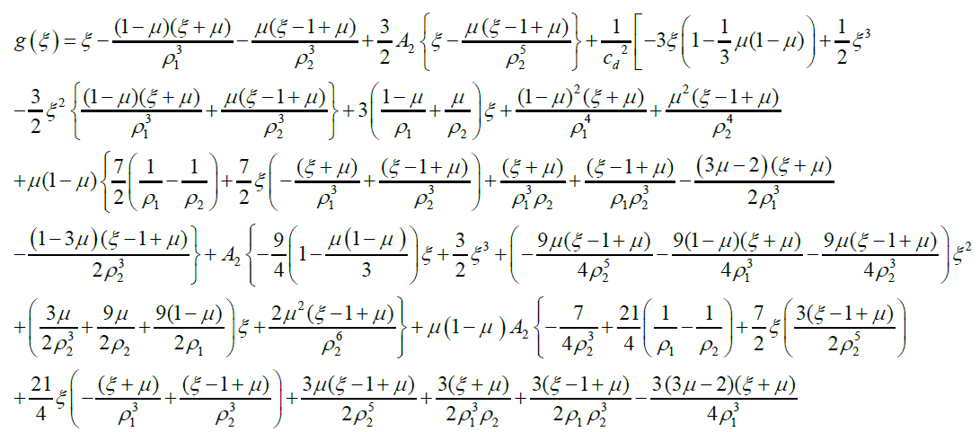
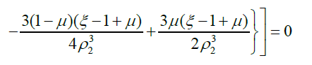 (6)
(6)
with 
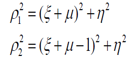
To locate the collinear points on the ξ − axis, we divide the orbital plane into three parts: ξ <ξ1 ,ξ1 <ξ <ξ2 and ξ2 <ξ 2 with respect to the primaries where ξ2 = 1−μ and ξ2= 1−μ
Case 1:
Position of L2 (ξ >ξ2 ) (see Figure. 1(a))

Figure 1: Reference parameter for collinear Lagrangian points.
Let  ; ; since the distance between the primaries is unity, i.e. and ξ2=1−μ then
 (7)
(7)
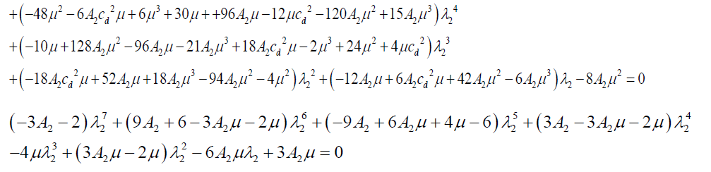
Now substituting equation (7) in (6), we obtain
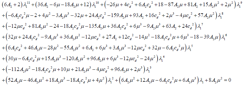 (8)
(8)
In the presence of oblateness effect only, we have
 (8a)
(8a)

Case 2: Position of ξ −ξ2 = λ2 ; (see Figure. 1(b))
Let  with ρi > 0(i =1,2) (9)
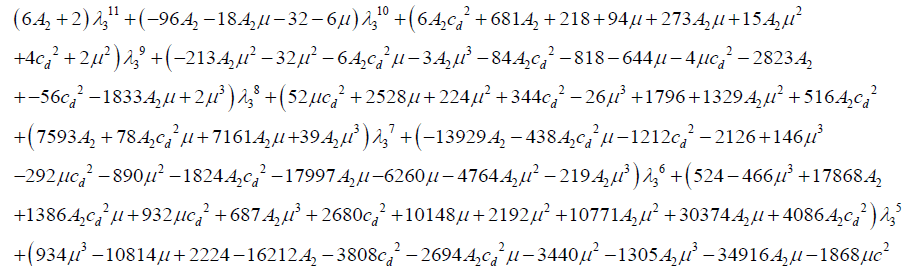
Substituting equation (9) in (6), we obtain:
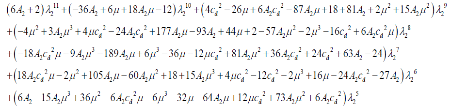 (10)
(10)
 (10a)
(10a)
In the presence of oblateness effect only, we have,
Case 3: Position of L3(ξ <ξ1) (see Figure. 1(c))
Let the distance of the point 1−λ from the bigger primary be 1−λ3
 with
with
ρi > 0(i =1,2) (11)
Substituting equation (11) in (6), we obtain,
 (12)
(12)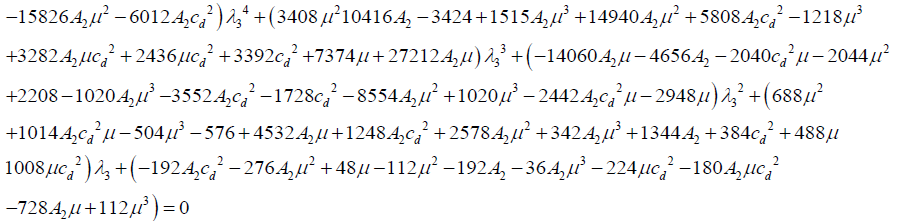
In the presence of oblateness effect only, we have,
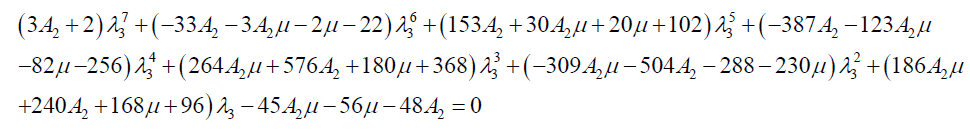 (12a)
(12a)
It is noticed that in each case there exists only one physically reasonable root.
Stability of collinear points
We examine the stability of an equilibrium configuration; that is, its ability to restrain the body motion in its vicinity. To do so we displace the infinitesimal body a little from an equilibrium point with a small velocity. If its motion is rapid departure from vicinity of the point, we call such a position of equilibrium an unstable one. If the body oscillates about the point, it is said to be a stable position.
In order to study the stability of the collinear points, following Singh and Bello [17] the characteristic equation is given by (13):
where,
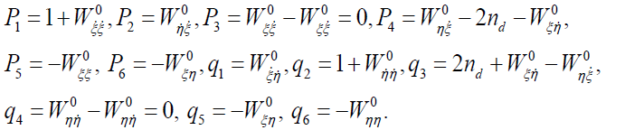 (13)
(13)
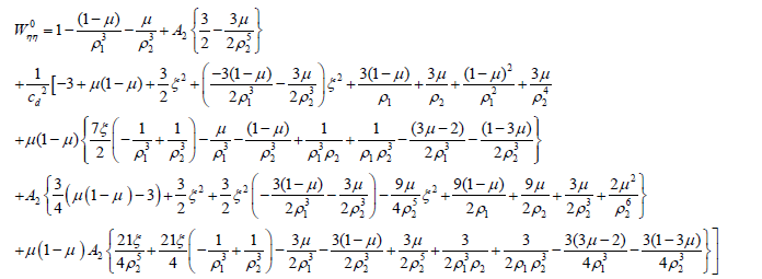
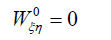
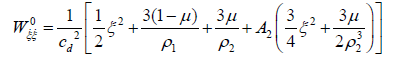
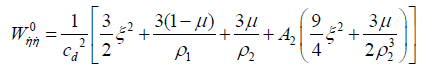
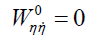
The second order partial derivative of 0 are denoted by subscripts. The superscript 0 indicates that the derivative is to be evaluated at the collinear equilibrium points (ξ0 ,η0) under consideration.
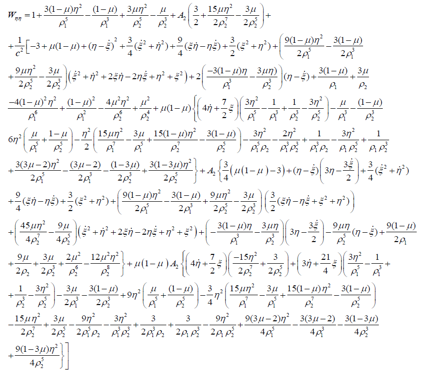
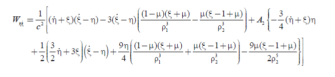
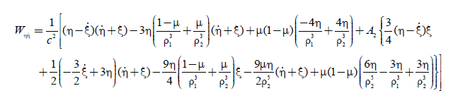
The second order derivatives are
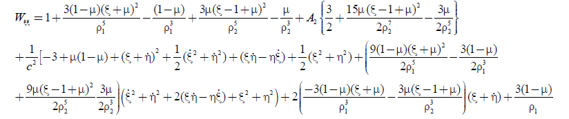
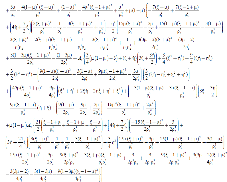 (14a)
(14a)
 (15a)
(15a)
 (16a)
(16a)
 (17a)
(17a)
 (18a)
(18a)
 (19a)
(19a)
 (20a)
(20a)
 (21a)
(21a)
In order to study the stability of the collinear points we have to study the motion in the proximity of these points, hence in this case (14a)-(21a) can be written as:
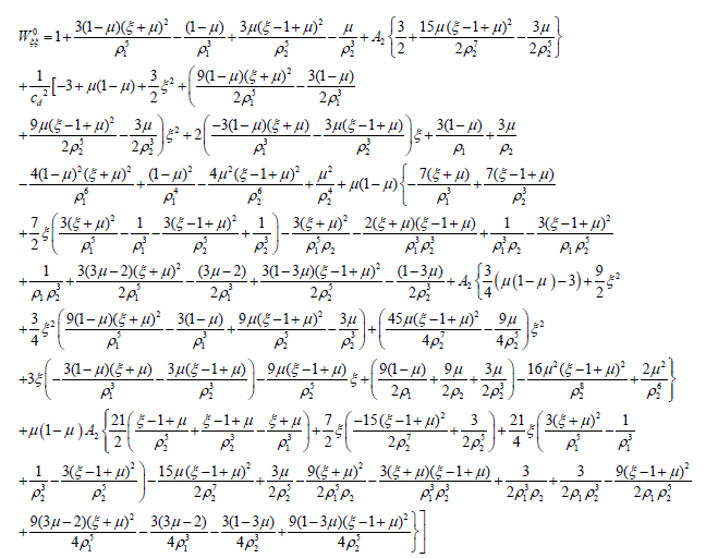 (14b)
(14b)
 (15b)
(15b)
 (16b)
(16b)
 (17b)
(17b)
 (18b)
(18b)
 (19b)
(19b)
 (20b)
(20b)
 (21b)
(21b)
Now we will show the discriminant Δ of (13) is positive at the collinear points Li (i =1,2,3)
To show Δ is positive it is sufficient to show that
 (25)
(25)
M can also be written as
From (17b) and (18b) it is clear that
Now we will study the signs of  and
and  at the collinear points Li (i =1,2,3)
Firstly, we will do this at L1, since the coordinates of this point is  , then ρ2=λ1 and ρ2=λ1 where 0 <λ1<<1, hence we can write
  and λ1 as a function of λ1
, say f (λ1),and f (λ1), respectively. In this case from (14b), h(λ1 ) ≅ h(0+ ) = −∞
and from (15b), f (λ1 ) ≅ f (0+ ) = +∞, hence
and λ1 as a function of λ1
, say f (λ1),and f (λ1), respectively. In this case from (14b), h(λ1 ) ≅ h(0+ ) = −∞
and from (15b), f (λ1 ) ≅ f (0+ ) = +∞, hence  and
and  contrary to the classical case where
 However
 and consequently
 , Hence the discriminant of the equation (13) is positive, and the characteristic roots can be written as
 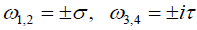 where σ and τ are real.
Thus ω1,2 are real and , L1 are pure imaginary, hence the motion around the collinear point , L1 is unbounded and the solution is unstable.
Similarly, it can be shown that the points L2 , L3 are also unstable.
Numerical Results
The necessary data used have been borrowed from Sharma and SubbaRao [4] and Ragos et al. [14]. We have used some members of the solar system (mentioned in Table 1) to examine the existence and position of the collinear equilibrium points. Equations (8), (10), (12) and (8a), (10a), (12a) have been solved for the various pairs of the solar system. In Table 2 we present the positions of collinear points of the Sun-Planet pairs of Table 1. We also include the corresponding positions respectively in the classical problem, classical problem with oblateness, relativistic problem and relativistic problem with oblateness for comparison purposes (first entry, second entry, third entry and forth entry respectively for each system).
| S. No | System | cd | μ | A2 |
|---|---|---|---|---|
| 1 | Sun-Earth | 10064.84 | 0.000003003500 | 0.0000000007× 10⁻⁸ |
| 2 | Sun-Mars | 12424.24 | 0.000000322700 | 0.0000000001× 10⁻⁸ |
| 3 | Sun-Jupiter | 22947.35 | 0.000953692200 | 0.0000192887× 10⁻⁸ |
| 4 | Sun-Saturn | 31050.90 | 0.000285726000 | 0.0000018690× 10⁻⁸ |
| 5 | Sun-Uranus | 44056.13 | 0.000043548000 | 0.0000000070× 10⁻⁸ |
| 6 | Sun-Neptune | 55148.85 | 0.000051668900 | 0.0000000010× 10⁻⁸ |
Table 1: Parameters of the systems.
| S/No of the system | L1 | L2 | L3 |
|---|---|---|---|
| 1 | 1.01003413809074 | 0.99002657245074 | -1.00000125145833 |
| 1.01003413809000 | 0.99002657245100 | -1.00000125145833 | |
| 1.01003413806000 | 0.99002657248500 | -1.00000125145831 | |
| 1.01003413806000 | 0.99002657248500 | -1.00000125145831 | |
| 2 | 1.00476303037278 | 0.99525140276082 | -1.00000013445833 |
| 1.00476303037300 | 0.99525140276100 | -1.00000013445833 | |
| 1.00476335306300 | 0.99525140276100 | -1.00000013445833 | |
| 1.00476335306300 | 0.99525140276100 | -1.00000013445833 | |
| 3 | 1.06882613997466 | 0.93236993769216 | -1.00039737170283 |
| 1.06882613998000 | 0.93236993769000 | -1.00039737170270 | |
| 1.06882613992000 | 0.93236993764000 | -1.00039737170120 | |
| 1.06882613992000 | 0.93236993764000 | -1.00039737170120 | |
| 4 | 1.04606932684648 | 0.95474919731454 | -1.00011905249873 |
| 1.04606932685000 | 0.95474919731000 | -1.00011905249870 | |
| 1.04606932683000 | 0.95474921600000 | -1.00011905249850 | |
| 1.04606932683000 | 0.95474921600000 | -1.00011905249850 | |
| 5 | 1.02454737494085 | 0.97576220621890 | -1.00001814499999 |
| 1.02454668140000 | 0.97576220622000 | -1.00001814499999 | |
| 1.02454668140000 | 0.97576220665000 | -1.00001814499998 | |
| 1.02454668140000 | 0.97576220665000 | -1.00001814499998 | |
| 6 | 1.02599374139930 | 0.97434749094956 | -1.00002152870832 |
| 1.02599374140000 | 0.97434749095000 | -1.00002152870833 | |
| 1.02599374140000 | 0.97434749156000 | -1.00002152870831 | |
| 1.02599374140000 | 0.97434749156000 | -1.00002152870831 |
Table 2: Positions of the collinear equilibrium points.
Discussion
Equations (1) - (4) describe the motion of a third body under the influence of the oblateness of the smaller primary and relativistic terms. Equations (8), (10) and (12) give respective positions of the collinear equilibrium points L1, L2 , L3 in the presence of relativistic and oblateness factors while equations (8a), (10a) and (12a) give their positions in the presence of oblateness factor only. It can be seen in section 4 that the relativistic and oblateness factors are unable to alter the instability behavior of the collinear points. It can be observed when comparing first and second entries of each Sun-Planet pair that the positions of L1 and L3 are affected by oblateness in the classical problem, while when comparing first and third entries it can be said that the presence of the relativistic terms affects them. It is also noticed that the oblateness effect on the position of the collinear point L3 of the classical problem in most of the cases is negligible when comparing first and second entries except for the Sun- Jupiter system where it has a little effect, while also when comparing first and third entries it can be said that the relativistic terms have negligible effect on the position of L1 except for the Sun- Jupiter and Sun- Saturn systems.
It is also noticed that the oblateness and relativistic factors have separately the same effect on the position of L1 of the Sun- Uranus system and have same separate effect on the position of L3 of the Sun-Neptune system as shown from second and third entries of those systems.
However, in all cases it is found that the third and fourth entries of the relativistic problem only and relativistic problem with oblateness respectively are same up to fourteen decimal places. This indicates that in the presence of relativistic terms, the effect of oblateness does not show physically on the positions of collinear points in our Solar system. It is also observed that all the parameters involved have no effect on the position of L3 of the Sun -Mars system.
Conclusion
By considering the smaller primary as an oblate spheroid, we have studied the positions of the collinear points and their linear stability in the relativistic R3BP. It is found that despite the inclusion of relativistic and oblateness coefficients, the instability behavior of the collinear points remains unaltered. A numerical survey of some members of the Sun-Planet pairs of our solar system reveals that the positions of L3 and L3 are significantly affected by the oblateness in the absence of relativistic factor and by also relativistic factor in the absence of oblateness ; while the position of L3 is negligibly affected by oblateness and relativistic factors in most of the cases and more specifically all the parameters involved have no effect on the position of L1 of the Sun-Mars system. It is observed that the oblateness and relativistic factors have same separate effect on the position of L1 of the Sun-Uranus system they have also same effect on the position of L1 of the Sun-Uranus system. It is also noticed that in the presence of relativistic terms, the effect of oblateness does not show physically in our solar system as comparing third and fourth entries of Table 2.
For the future work, the effect of mass ratios on the locations and stability of collinear points are suggested.
References
- Szebehely V. Theory of orbits. The restricted problem of three bodies. Academic Press. New York; 1967.
- Renzetti, G. Exact geodesic precession of the orbit of two-body gyroscope in geodesic motion about a third mass. Earth-Moon and Planets. 2012;109(1-4):55-9.
- Iorio L. An assessment of the systematic uncertainty in present and future tests of the Lense-Thirring effect with satellite laser ranging. Space Sci Rev. 2009;135:271-81.
- Sharma RK, Subba-Rao PV. Collinear equilibria and their characteristics exponents in the restricted three-body problem when the primaries are oblate spheroids. Celestial Mechanics.1975;12:189-201.
- Oberti P, Vienne A. An upgraded theory for Helene, Telesto, and Calypso. Astronomy and Astrophysics. 2003;397:353-59.
- Abouelmagd, EI. Existence and stability of triangular points in the restricted three-body problem with numerical applications. Astrophys Space Sci. 2012;342,45-53.
- Abouelmagd, EI. Asiri HM, Sharaf MA.The effect of oblateness in the perturbed restricted three-body problem. Meccanica, 2013;48:2479-2490.
- Singh J, Umar A. On the stability of triangular equilibrium points in the elliptic R3BP under radiating and oblate primaries. Astrophys Space Sci. 2013;341:349-58.
- Brumberg VA. Relativistic celestial mechanics. Nauka Moscow; 1972. 384p.
- Brumberg VA. Essential relativistic celestial mechanics. Adam Hilger;1991. 271p.
- Bhatnagar KB, Hallan PP. Existence and stability of in the relativistic restricted three-body problem. CelestMechDynAstron. 1998;69:271-81.
- Douskos CN, Perdios EA. On the stability of equilibrium points in the relativistic restricted three-body problem. Celest. MechDyn Astron. 2002;82:317-21.
- Ahmed MK, Abd El- Salam FA. Abd El- Bar SE. On the stability of triangular Lagrangian equilibrium in the relativistic restricted three-body problem. Am J Appl Sci. 2006;3:1993-998.
- Ragos O,Perdios EA,Kalantonis VS, et al. On the equilibrium points of the relativistic restricted three- body problem. Nonlinear Anal. 2001;47:3413-418.
- Abd El-Bar SE, Abd El-Salam FA. Analytical and semi-analytical treatment of the collinear points in the photo gravitational relativistic RTBP. Math. probl. Eng. 2013.
- Abd El-Salam FA, Abd El-Bar SE. On the triangular equilibrium points in the photo gravitational relativistic three-body problem. Astrophys Space Sci. 2014;349:125-35.
- Singh J, Bello N. Motion around in the perturbed relativistic R3BP. Astrophys Space Sci. 2014a;351:491-97.
- Singh J, Bello N. Effect of radiation pressure on the stability of in the relativistic R3BP. Astrophys Space Sci. 2014b; 351483-90.
- Katour DA, Abd El-Salam FA, Shaker MO. Relativistic restricted three-body problem with oblateness and photo gravitational corrections to triangular equilibrium points. Astrophys Space Sci. 2014;351(1):143-49.
- Bello N,SinghJ. On the stability of triangular points in the relativictic R3BP with oblate primaries and bigger radiating. Adv Space Res. 2016;57:576-87.
- McCuskey SW. Introduction to celestial mechanics. Addison-Wesley;1963.