Original Article
, Volume: 5( 4)Frequency analysis of short periodic Cepheid BD+13 218 as Seen from SMEI Observations
- *Correspondence:
- Abdel-Sabour MR Dept Of Physics and astronomy, faculty of science, King Saud University, Al Riyadh, Saudi Arabia, Tel: +972 1-800-660-660; E-mail: sabour2000@hotmail.com
Received Date: July 6, 2017 Accepted Date: September 26, 2017 Published Date: October 06, 2017
Citation: Abdel-Sabour MR. Frequency analysis of short periodic Cepheid BD+13 218 as Seen from SMEI Observations. J Phys Astron. 2017;5(4):120
Abstract
A total of 1848 flux observations of BD+13 218 are obtained by using the Solar Mass Ejection Imager (SMEI) on board of the Coriolis satellite. The data reveal a significant cycle-to-cycle fluctuation in the pulsation period, indicating that classical Cepheid may not be accurate regardless of the specific points used to determine the O-C values. Eddington & Plakidis (1929) methods and random fluctuations in periods were studied. The present detailed O-C residuals for pulsating star BD+13 218 (P=2.8364 day) is studied. Pulsation frequencies and Fourier spectra are presented. By using the empirical relations for stellar structure we determined the parameters of BD+13 218, Teff = 5917.052±145.262,
Keywords
Stars; Evolution – stars; Individual; BD+13 218 – Cepheids
Introduction
For over one hundred years, variable stars have been used as probes of astronomical distances and stellar physics. To this day, they continue to be at the forefront of modern astrophysics. [1] remarks that type II Cepheids ‘‘include most intrinsic variables with periods between 1 and about 50 days, except for the classical Cepheids and the shortest semiregular variables of type M.’’ These bounds on the periods place the type II Cepheids in the instability strip between the RR Lyrae stars at the short-period limit and the RV Tau variables at the long-period limit. Type II Cepheids fall into two classes: BL Her stars with periods of 1- 5 days and the W Vir stars with periods longer than about 10 days, with an indistinct boundary at about 20-30 days separating these stars from the RV Tau stars. [2] drew attention to the period gap (6-9 days) between the BL Her and W Vir stars in globular clusters. On the average Pop II are about 1.5 mag fainter than Pop I of the same period. There are three subclasses of Pop II in different stage of evolution. BL Her stars have the shortest period and are evolving from the horizontal branch to word asymptotic giant branch (AGB). The rate of observed period changes is in a good agreement with that determined from stellar evolution theory. The number of stars in first, second and third crossing of the instability strip, on the basis of the derived rates of period change, are not fully consistent with time scales based upon stellar evolution cross the inferred width of the strip. There are fewer stars in fifth crossing than predicted on that basis, and fewer at long period, may be because not all massive stars cross the instability strip during the period of shell helium burning.
For that we try to put one variable star (BD+13 218) under focus hopping to have new results, especially after the observations we get from Solar Mass Ejection Imager (SMEI).(SMEI) is the unique data set of continuous monitoring of the entire sky which has been used to study variations in the brightness of stars. Photometric data from SMEI have already been used for studying the period and amplitude evolution of Polaris by [3]. The reader is referred to Spreckley & Stevens [3] for a detailed description of the data extraction and processing pipeline.
The primary aim of the present investigation is to test whether the observed times of maxima or minima are consistent with the hypothesis that the Irregularities are the individual period may differ from the mean period by a purely accidental fluctuation independent of previous fluctuations.
We present the data technique and reduction in section 2. Also, we describe the O-C properties and period change for our system BD+13 218 in sec. 3. A Fourier decomposition technique using an algorithm for non-linear least square fitting is studied in Sect.4. The physical properties of our system are described in more detail in sect.5. Finally, in Sect. 6, we presented important conclusions of the study.
Data and Method of Analysis
Due to the lack of the continuous observations of the star BD+13 218, our study will depend on the observations available from ASAS (http://www.astrouw.edu.pl/asas/) and SMEI databases.
SMEI instrument is launched on 2003 January into an 840-km sun-synchronous polar orbit with an orbital period of 101 min. More description of SMEI data was presented by [3] and details on the SMEI instrument was presented by [4].
Both these data allow us to construct many consecutive individual light curves, and to search for random fluctuations in period and amplitude for BD+13 218 Cepheid variable.
SMEI observations are analyzed using the Period04 software and other Fortran program for a comprehensive investigation of their pulsation properties.
BD+13 218 Star
BD+13218 (GSC 00620-00985), (α2000=01:28:37.9 & δ2000=14:39:29.9) and, B=10.63 ± 0.05, V=9.63 ± 0.03, J=7.657 ± 0.020, H=7.178 ± 0.038, K=7.089 ± 0.023, Photometry conducted by the authors revealed a period of P=2d.8364 and a peak-to-peak amplitude of 0.474 mag. In spite of, Simbad website descript the star as classical Cepheid, but we think this star lie under Pop II (BL Her), because Classical pulsating stars are Luminous, F-and G type, with periods from a few days up to 100 d.
The SMEI observations for this star started from 1 April, 2007 to 6 February 2010, see Figure 1. In our study, we used the resulting linear ephemeris which given by: JDmax= 2454191.501+2.8364E and/or JDmin= 2454528.65+2.83647E, where E is the number of elapsed cycles. Data were analyzed for periodicities with the PERIOD04 package (Lenz & Breger 10-15). The periodogram of the whole Camera #2 dataset is shown in Figure 2

Figure 1: SMEI observation for BD+13 218 pulsating variable, as seen four panels as a result of the gap between observations. First started from 1 to 9Abril 2007, the second 28 Feb to 19 March 2008, the third 7 Feb to 26 Feb 2009, and the forth started from 19 Jan to 6 Feb 2010.

Figure 2: High-precision photometric data from SMEI taken between April 2003 and March 2006 were subjected to periodogram analysis with the PERIOD04 package.
Period Change In BD+13 218
To study period change with acceptable accuracy, we should have observations on a long run. But we try to study the period change by using the data which we have. We studied the period stability of BD+13 218 applying the classical O−C diagram method. Observations of SMEI enable us to determine the O−C values for almost all cycles available. We used two different methods to calculate the O−C values.
The first one use SMEI observation only by using the times of maxima and minima of the light curves by two software’s (AVE and Minima), So O−C diagrams can be seen in Table 1 and Figure 3.

Figure 3: The O-C and Residual for the Time of maxima and minima light, by using SMEI observations.
| Time of maximum | Time of minimum | ||||||
|---|---|---|---|---|---|---|---|
| Tmax. | Err. | Epoch | O-C | TMin. | Err. | Epoch | O-C |
| 2454192.550 | 0.014 | 0.000 | 0.00097 | 2454193.911 | 0.012 | 0.480 | -0.05158 |
| 2454195.313 | 0.026 | 0.974 | -0.06290 | 2454195.461 | 0.104 | 1.027 | -0.08530 |
| 2454198.220 | 0.016 | 1.999 | -0.01830 | 2454525.781 | 0.032 | 117.485 | -0.28805 |
| 2454527.238 | 0.010 | 117.999 | -0.24433 | 2454528.661 | 0.011 | 118.501 | -0.23477 |
| 2454530.093 | 0.007 | 119.006 | -0.21606 | 2454531.381 | 0.025 | 119.460 | -0.34098 |
| 2454532.911 | 0.005 | 119.999 | -0.22415 | 2454534.263 | 0.013 | 120.476 | -0.28550 |
| 2454535.739 | 0.016 | 120.996 | -0.22311 | 2454537.093 | 0.010 | 121.473 | -0.28240 |
| 2454538.557 | 0.012 | 121.990 | -0.23146 | 2454539.988 | 0.015 | 122.494 | -0.21302 |
| 2454541.380 | 0.020 | 122.985 | -0.23458 | 2454542.659 | 0.018 | 123.436 | -0.36897 |
| 2454544.013 | 0.073 | 123.913 | -0.42825 | 2454871.896 | 0.011 | 239.513 | -0.41272 |
| 2454870.423 | 0.008 | 238.993 | -0.47194 | 2454874.677 | 0.010 | 240.493 | -0.45772 |
| 2454873.290 | 0.012 | 240.004 | -0.43138 | 2454877.517 | 0.015 | 241.494 | -0.44440 |
| 2454876.088 | 0.012 | 240.991 | -0.46042 | 2454879.857 | 0.004 | 242.320 | -0.48291 |
| 2454878.941 | 0.010 | 241.997 | -0.43316 | 2455215.027 | 0.011 | 360.488 | -0.27738 |
| 2454881.773 | 0.021 | 242.995 | -0.42784 | 2455217.923 | 0.021 | 361.509 | -0.34070 |
| 2454884.685 | 0.024 | 244.022 | -0.34216 | 2455220.652 | 0.013 | 362.471 | -0.47246 |
| 2454887.456 | 0.016 | 244.999 | -0.39734 | 2455223.582 | 0.014 | 363.504 | -0.69388 |
| 2455216.461 | 0.020 | 360.994 | -0.67381 | 2455226.401 | 0.022 | 364.498 | -0.62488 |
| 2455219.328 | 0.015 | 362.005 | -0.63249 | 2455231.972 | 0.027 | 366.462 | -0.69144 |
| 2455222.131 | 0.010 | 362.993 | -0.65641 | 2454880.510 | 0.024 | 242.550 | -0.61859 |
| 2455224.992 | 0.019 | 364.001 | -0.62156 | 2454883.273 | 0.016 | 243.524 | -0.62605 |
| 2455227.798 | 0.009 | 364.991 | -0.64180 | 2454885.968 | 0.017 | 244.474 | -0.70506 |
| 2455230.633 | 0.014 | 365.990 | -0.63396 | -- | -- | -- | -- |
| 2455233.295 | 0.023 | 366.929 | -0.61501 | -- | -- | -- | -- |
Table. 1. Period change in Bd+13 218
The average error of the time of maxima/minima is ± 0.060 d, which was determined by applying this method to a synthetic light curve generated using the Fourier parameters of BD+13 218 and averaging the deviations between the analytically derived maxima/minima.
Determining the O-C by studying the time of maximum or minimum is not easy because sometimes the maxima or minima of light curve are not well defined by the data as a result of scattering observations. Thus, at this point it is not always possible to determine a precise O-C by using phase shift. The average measurements are fairly consistent with the period change log P(dot)=1.853 ± 0.266 s/yr.
The second method to studying the O-C are plotted in Figure 4 Which used by measure phase shifts of each cycle and transforms them to an O−C diagram. The phase folded light curves containing data from January 2003 to January 2010.

Figure 4: The O–C diagram as a constant period, the slop line is to the estimated period change (above panel) and Residual (down panel) Data Obtained by using the second method. By using all data available.
The O-C data are matched reasonably closely by a parabola form HJDmax=Mo+PE+QE2 which indicative of a regular period change described by ;
Where E is the number of elapsed cycles. Then the inferred rate of period changes for BD+13 218 is 1.826 ± 0.213 s/y. this rate of period change almost exactly what one predicts for a star in the first crossing of the instability strip as seen in Figure 5. Figure 5 depicts some of the best-established rate of period change as a function of the pulsation period for a selection of variable undergoing increases, [5] and [6]. The plots relations for first, third, and fifth crossings of the instability strip were derived from published evolutionary model by [7] (sold, dashed and dot lines in Figure 4, Figure 5). Comparison between the theoretical evolutionary mode [7] and observations reveals that, BD+13 218 is the first crossing of the instability strip as seen from Figure 6, more observations is needed to confirm this result. Table. 2

Figure 5: Rates of period change as a function of the pulsation period for a sample of variable with established period increasing, with error bars denoting the uncertainties in derived quantities.

Figure 6: The <U(x)>2 diagram for U Aql, η Aql, ξ Gem, X Lac, T Mon, T Vul, and BD+13 218.
| JD | Epoch | O-C | Weight | No. | Ref. |
|---|---|---|---|---|---|
| 2452649.722 | 3 | 7.213 | 2 | 11 | ASAS |
| 2452917.637 | 98 | 5.67 | 1 | 47 | ASAS |
| 2452999.975 | 127 | 5.752 | 2 | 12 | ASAS |
| 2453312.583 | 238 | 3.52 | 2 | 12 | ASAS |
| 2453631.999 | 350 | 5.259 | 1 | 32 | ASAS |
| 2453729.018 | 385 | 3.004 | 1 | 14 | ASAS |
| 2453848.800 | 428 | 3.833 | 2 | 36 | SMEI |
| 2454195.438 | 550 | 1.418 | 3 | 217 | SMEI |
| 2454384.501 | 616 | 3.279 | 2 | 53 | ASAS |
| 2454534.984 | 670 | 0.596 | 3 | 540 | SMEI |
| 2454756.915 | 748 | 1.288 | 1 | 53 | ASAS |
| 2454879.337 | 792 | -1.092 | 3 | 554 | SMEI |
| 2455094.058 | 867 | 0.899 | 2 | 25 | ASAS |
| 2455217.875 | 911 | -0.085 | 3 | 74 | SMEI |
| 2455223.647 | 913 | 0.014 | 3 | 513 | SMEI |
Table. 2. Observations is needed to confirm this result
Random Cycle To Cycle Period Fluctuations
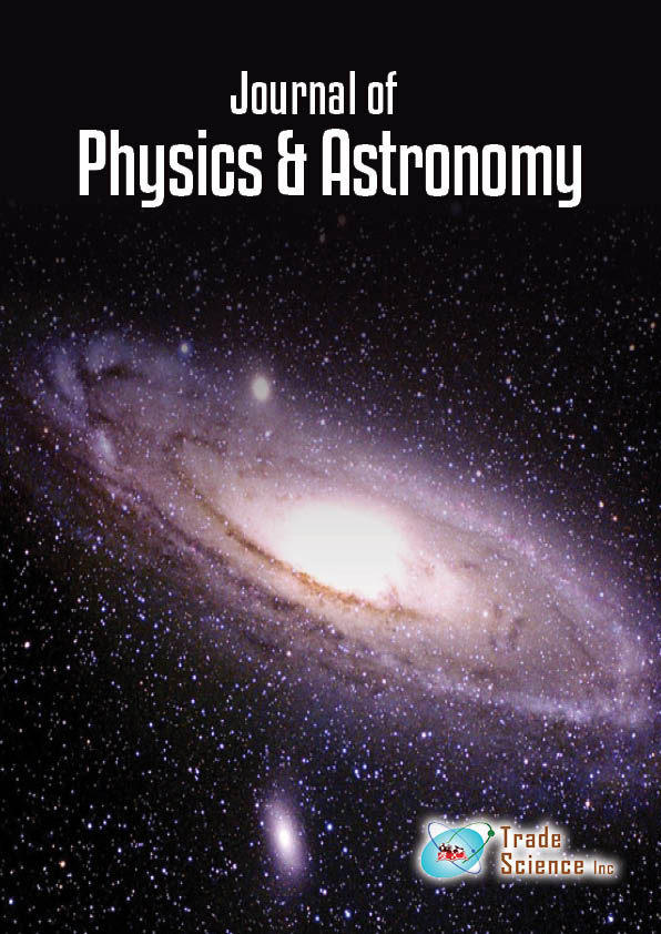
Random fluctuations must present in periods of all pulsating variables. A test to detect these fluctuations was proposed by [8]. If the O-C diagram are affected by random errors in the measurement times of maximum or minimum, and if these quantities are accidental and uncorrelated, then a graph of <u(x)>2 versus of x is a straight line, where x is a number of cycles between (O-C), and <u(x)> is the average absolute value of the differentness between all pairs of O-C diagrams that are x cycles apart [9] i.e the accumulated delays <U(x)>=average  between maxima separated by x cycles. By the ordinary theory of errors, the probable value of the sum of x fluctuations is
  times the probable value of one fluctuation. If the deviations in observed time of maxima from their predicted times are dominated by random fluctuations in period, then that data for all available observed light maxima should display a trend described by:
where “a” is the average uncertainty in days for established times of light maxima and “e” is the magnitude of some random fluctuation in period. A schematic representation of expectation for pulsating variable is presented in Fig. 6 for our system and the other taken from [8] The weighted least square fit to the u(x)2 data from our system (BD+13 218) is:

with SIGMA = 0.00231 where the null value of the slope of the relation is consistent with no random cycle- to-cycle fluctuation in period for BD+13 218 at least for the observations that we used. The observed values of, <u(x)>2 therefore become very small for large cycle differences. Convincing evidence for random cycle- to-cycle variations in pulsation period for several different types of long period variables was published by [9]. For these variables, the existing observations allowed us to construct many consecutive individual light curves. Since random fluctuations in period exist in the time
interval of several to a few tens of pulsation cycles, it is easy to be detected for about two hundred stars. In the case of galactic variable whose periods are shorter than 68 days, such dense series of observations did not exist and random fluctuations were found only in a period in about ten variables which have long period observations Figure 6.
Fourier Decomposition Method
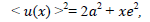
The principal component analysis (PCA) and Fourier decomposition (FD) method are an important tool for variable star light curve analysis and compare their relative performance in studying the changes in the light curve structures of pulsating variable and in the classification of variable stars. The light curves are fitted with the following formula [10].
where m (t) is the magnitude observed at time t , m0 is the mean magnitude Ai is the amplitude of the i- component (harmonic), f is the frequency (f = 1/P, where P is the period of the light variation), φi is the phase of the i-component. The Fourier parameters can be subdivided into two groups: the amplitude ratios and the phase differences φy = iφj - jφi We calculate Fourier coefficient because the larger value of R21indicates stronger deviations from a single sinusoid and thus indicates a higher degree of asymmetry in the light curve. Table 3 lists the calculated Fourier parameters. Fig. 6 plots the amplitude stability. The least square fit of SMEI observation is:
| Mean. JD. | A1 | R21 | R31 | phi21 | phi31 | No. |
|---|---|---|---|---|---|---|
| 2454192.765 | 0.506 ± 0.025 | 0.112 ± 0.034 | 0.107 ± 0.04 | 1.885 ± 0.493 | 2.204 ± 0.324 | 88 |
| 2454198.726 | 0.472 ± 0.037 | 0.175 ± 0.083 | 0.065 ± 0.08 | 2.475 ± 0.431 | 1.911 ± 1.166 | 71 |
| 2454526.346 | 1.123 ± | 0.967 ± 0.144 | 0.800 ± 0.29 | 5.589 ± 1.474 | 4.557 ± 2.306 | 52 |
| 2454528.763 | 0.510 ± 0.011 | 0.113 ± 0.021 | 0.119 ± 0.02 | 1.884 ± 0.203 | 2.822 ± 0.203 | 74 |
| 2454531.434 | 0.473 ± 0.022 | 0.066 ± 0.033 | 0.088 ± 0.03 | 0.443 ± 0.589 | 3.659 ± 0.427 | 73 |
| 2454534.236 | 0.488 ± 0.014 | 0.120 ± 0.028 | 0.043 ± 0.03 | 1.879 ± 0.255 | 2.639 ± 0.674 | 90 |
| 2454537.242 | 0.501 ± 0.015 | 0.081 ± 0.03 | 0.121 ± 0.03 | 0.633 ± 0.381 | 3.093 ± 0.267 | 98 |
| 2454540.153 | 0.429 ± 0.020 | 0.022 ± 0.046 | 0.095 ± 0.05 | 4.344 ± 2.002 | 2.959 ± 0.459 | 79 |
| 2454542.930 | 0.599 ± 0.042 | 0.279 ± 0.063 | 0.149 ± 0.06 | 0.758 ± 0.201 | 2.084 ± 0.374 | 70 |
| 2454871.609 | 0.525 ± 0.010 | 0.139 ± 0.019 | 0.062 ± 0.02 | 1.292 ± 0.154 | 3.754 ± 0.316 | 102 |
| 2454874.729 | 0.460 ± 0.012 | 0.139 ± 0.026 | 0.063 ± 0.02 | 1.857 ± 0.183 | 3.010 ± 0.415 | 83 |
| 2454877.545 | 0.496 ± 0.015 | 0.115 ± 0.029 | 0.082 ± 0.03 | 1.705 ± 0.235 | 3.132 ± 0.317 | 81 |
| 2454880.335 | 0.479 ± 0.016 | 0.176 ± 0.034 | 0.018 ± 0.03 | 2.431 ± 0.197 | 3.773 ± 1.862 | 88 |
| 2454883.112 | 0.488 ± 0.021 | 0.151 ± 0.042 | 0.151 ± 0.04 | 1.088 ± 0.302 | 3.772 ± 0.313 | 89 |
| 2454886.869 | 0.473 ± 0.028 | 0.157 ± 0.063 | 0.064 ± 0.07 | 2.370 ± 0.362 | 1.503 ± 0.975 | 111 |
| 2455220.720 | 0.422 ± 0.015 | 0.179 ± 0.032 | 0.112 ± 0.03 | 1.829 ± 0.176 | 2.373 ± 0.290 | 77 |
| 2455227.364 | 0.443 ± 0.012 | 0.173 ± 0.028 | 0.037 ± 0.03 | 1.564 ± 0.167 | 3.623 ± 0.743 | 311 |
Table. 3. The SMEI Fourier parameters of the light curve fitting
YSMEI= -1.6322E-006*X+4.4813, R-squared = 0.002, sigma= 0.0003,
and for ASAS Observations is;
YASAS=-1.454E-005*X+35.795, R-squared = 0.119, sigma= 0.0012.
Physics Parameters
In this section, we present a set of functional relationships that allow us to derive the atmospheric parameters using the intrinsic colors as independent variables in the infrared or visible regions. We use both regions but we know infrared colors are less subject to the effects of interstellar absorption. We try to calculate the physical parameters for BD+13 218, Effective temperature (Teff), absolute magnitude Table 4
| Mean. JD | Amp. | Err | R21 | Err | R31 | Err | φ21 | Err | φ31 |
|---|---|---|---|---|---|---|---|---|---|
| 2454195.745 | 0.489 | 0.031 | 0.144 | 0.059 | 0.086 | 0.059 | 2.180 | 0.462 | 2.057 |
| 2454535.793 | 0.487 | 0.021 | 0.114 | 0.037 | 0.103 | 0.037 | 1.657 | 0.605 | 2.876 |
| 2454879.033 | 0.488 | 0.017 | 0.146 | 0.035 | 0.073 | 0.037 | 1.791 | 0.239 | 3.158 |
| 2455224.042 | 0.432 | 0.013 | 0.176 | 0.030 | 0.075 | 0.029 | 1.697 | 0.172 | 2.998 |
Table. 4. Amplitude stability for BD+13 218, dot points is the SMEI observations, asters points is the ASAS observation
 and surface gravity (log g). In the following subsection we have used the constants adopting, Teff sun =5777 K, log g?=4.44, Mbol?= 4.75, )V-R(*= 0.622, (H-K)* = 0.089 and (J-H)* = 0.479.
Effective Temperature
There were two camps for effective temperatures of BD+13 218, one claiming the temperature is 4420K, 4581 K by [11,12] , respectively, and the other claiming is the effective temperature in the rang (6311-6385)k by [3]. The large difference between the two results may be attributed to that, the first one is calculated it when the star expanded and the second’s calculated when the phase of the star compresses. So we used her the Temperature from [3] and rejected the temperature from [11,12] because we try to calculated it’s by empirical formula and the our results close to the [3].
We know determining the stellar effective temperature from color or spectra is a difficult task. The photometric angular diameters derived using the color index (B-V) fails to predict the correct temperature of pulsating star during the expansion phase. So, we use the infrared region as a functional relationship involving the intrinsic colors (J−H)0 , because the infrared colors are less subject to the effects of interstellar absorption. By using the formula by [2,13-15] and the results is around 5917.052±145.262 K. But, we depend to calculated the following parameters to the effective temperature from [3].
Radius
The stellar radius is calculated from a polynomial fit to the temperature-radius relation given by Collier Cameron et al.[13], which is valid for the temperature range 4000k <Teff < 7000k. also Gray (1992,eq. [15.14]) which give us the relation between effective temperature Teff and broadband (B- V)0 color. Many authors studied the Period-Radius relation [16-18,20,6] but the best-fitting relation obtained from a combination of least squares, weighted least squares, and nonparametric techniques is ;

see comments by [18,19]. We depend her about period-radius relation to determine the radius of the star under focus which give us 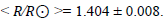
Mass and Surface Gravity
The stellar mass is then estimated by mass– radius and the surface gravity relationship as seen in the following equation from [21]
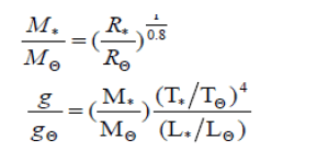
The results are M/M? = 1.528±0.087 and log g * = 2.284 ± 0.063.
Conclusion
Total 1824 flux magnitude estimates for pulsating star BD+13 218 is very important essential for understanding the initial vision of this star. The behavior of this star is so slow and complex and there are so many types of long-term variation, that the visual observations previous the only hope for further understanding. The longer the observation, the better our change of understanding will be.
-Time of minima and time of maxima was determined by using public software and the results are tabulated in Table 1.
The new results obtained with SMEI strongly suggest that the amplitude of BD+13 218 is stable.
The information about period changes is also presented as a phase diagram instead of a classical O–C diagram. Various shapes of the O–C curves correspond to following different cases:
If the period of the star is constant, but the adopted period is too long or too short, the straight line will slip up or down (see Fig. 3 &4). If dp/dt > 0, that is the O–C line will slop downwards and otherwise, dp/dp < 0, slop upwards. It tells us a shift in the epoch [20-24].
The period change noise is a result of random mixing events associated with the semi-convective zone of the stellar core [4].
From theoretical evolutionary model and observations, we see the star BD+13 218 is the first crossing of the instability strip as seen from Figure 5. And the period change rate estimate is 2 s/yr.
The star does seem to be oscillating in the first overtone mode, but likely lies close to the red edge of the instability strip, and is therefore likely to soon evolve into either a fundamental or double-mode variable, assuming the BD+13 218 is undergoing its first or third crossing.
Studying random fluctuation period, it is clearly understood the importance of the star’s period to the magnitude of the stochastic processes producing the random fluctuations in period.
Physical Properties for BD+13 218 are studied theoretically, effective temperature, luminosity, radius, stellar mass, surface gravity values which tabulated in Table 5 Recent, trends in the derived BW radii of Cepheids have consistently yielded values that lie close to the relationship obtained here. The transformation of Cepheid radii into luminosities requires the use of an effective temperature relation and a scale of bolometric corrections and generates Cepheid luminosities as absolute visual magnitudes MV.[24-26]
| Log Teff | L/L | R/R | (B-V)o | M/M | Log g |
|---|---|---|---|---|---|
| 3.802 | 0.386 | 1.404 | 1.044 | 1.528 | 2.24 |
Table. 5. The physical and observational properties of variable star BD+13 218.
Also, we hope to have photometric and spectroscopic data for BD+13 218 to study of the physical properties by very high accuracy.
Acknowledgements
I would to thank Ian Stevens for support me the SMEI data, M. Nouh and M. Elkhateep for revision and their advice.
References
- Turner, David G, Horsford. Ginsberg V Harry Eden Cross-Defendant And Appellant. Wallerstein. 2002;114: 689.
- Kathryn FN, Philip Massey, Brian Skiff. Travelling sexualities, circulating bodies, and early modern Anglo-Ottoman encounters. 2012;749: 12/ Kraft P. A Search for Small-Amplitude Spectroscopic Binaries among Main-Sequence FType Stars. Dudley Obs Rep. 1972;4: 2.
- Schmidt EG, Rogalla D, Thacker-Lynn L. PHOTOMETRY OF TYPE II CEPHEID CANDIDATES FROM THE NORTHERN PART OF THE ALL SKY AUTOMATED SURVEY. 2011;141: 53/ Spreckley, Stevens. Is Shedir Variable? MNRAS. 2008;388: 1239.
- Sweigart AV and Renzini A. Semiconvection and period changes in RR Lyrae stars. A&A. 1979;71:66/Tarrant NJ. Solar-like oscillations in low-luminosity red giants: first results from Kepler. A&A. 2008;492: 167-169.
- Sabour AM. Efficacy of bacteriophage LISTEX™ P100 combined with chemical antimicrobials in reducing Listeria monocytogenes in cooked turkey and roast beef. ROAJ. 2007;17: 109.
- Turner, David G, Horsford. Monitoring Cepheid Period Changes From Saint Mary's University. AAVSO. 1999;27: 5/ Wallerstein G. Synthesis of the elements in stars: forty years of progress. PASP. 2002;114; 689.
- Turner D. Conglomerate Mergers and Section 7 of the Clayton Act. AAVSO. 1998;26: 101.
- Eddington AS. Theory of relativity. MNRAS. 1929;90: 65.
- Percy J and Jonathan H. A DNA barcode for land plants. PASP. 1998;110: 1428.
- Petersen JO. Masses of double mode cepheid variables determined by analysis of period ratios. Astr Ap. 1984;139:496.
- Wright, Candace O, Egan. The Tycho-2 spectral type catalog. AJ. 2003;125: 359.
- Ammons SM, Robinson SE, Strader J, et al. The N2K Consortium VII Atmospheric Parameters of 1907 Metal-Rich Stars: Finding Planet-Search Targets. APJ. 2006;638: 1004.
- Collier Cameron A, Wilson D, et al. The WASP project and the SuperWASP cameras. Astronomical Society of the Pacific. 2006;118: 848.
- Alonso A, Arribas S, Martinez-Roger C. The effective temperature scale of giant stars (F0–K5) - II. Empirical calibration of versus colours and [Fe/H]. A&A. 1996;313: 873/ Alonso A, Arribas S, Martínez-Roger C. Alterations in structure and mechanics of resistance arteries from ouabain-induced hypertensive rats. A&ASS. 1999;140: 261.
- Lenz P, Breger M. Communications in Asteroseismology. RevMexAA. 2005;146: 53/ Molina RE. The ATLAS experiment at the CERN large hadron collider. RevMexAA. 2012;48: 95.
- Fernie JD. A database of Galactic classical Cepheids. ApJ. 1984;282: 641.
- Laney CD, Stobie RS. Cepheid period–luminosity relations in K, H, J and V. MNRAS. 1995;274: 337.
- Gieren WP, Fouque P, Gomez M. Cepheid period-radius and period-luminosity relations and the distance to the Large Magellanic Cloud. ApJ. 1998;496:17.
- Ripepi V, Barone F, Milano L, et al. Cepheid radii and the CORS method revisited. A&A. 1997;318: 797.
- Boyajian, Tabetha S, Kaspar von Braun. Stellar diameters and temperatures. II. Main-sequence K-and M-stars. The Astrophysical Journal. 2012;757: 2.
- Alcock C, Allsman RA, Alves DR., et al. The MACHO project: microlensing results from 5.7 years of large magellanic cloud observations. APJ. 2000;536:798.
- J Robert P, Laszlo Sturmann JS, Nils H Turner, et al. Infrared images of the transiting disk in the [epsilon] Aurigae system. ApJ. 2012; 57: 112.
- Breger M. Nonradial pulsation of the delta-scuti star Bu-Cancri in the praesepe cluster. A&A. 1990;240: 308.
- Clarkson DJ, Enoch WI, Esposito B, et al. Efficient identification of exoplanetary transit candidates from SuperWASP light curves. Astronomical Society. 2007;380: 1230-1244.
- Horne K, Irwin J, Kane SR, et al. The WASP project and the SuperWASP cameras. MNRAS. 2007;380: 1230.
- Philip Kaaret, Sabour AM, Ibrahim AA. Second international handbook on globalisation, education and policy research. RoAJ. 2015;25: 157.